The gaming industry is one of those industries that is chock full of technology and future probabilities. The reason is the component, platforms and objectives of a single game include various components made using technology and logic. With this amount of technology implementation in the industry, we can easily say that it is a compulsion for these technologies to include AI with them. The primary purpose of applying AI in gaming is to make the games more responsive and provide flexible game experiences to users.
The reality is that AI is what makes video or computer games more challenging and brings life to virtual games. In simple words, nowadays, AI environments are incorporating both virtual and augmented reality so that the future of gaming can become more robust and efficient. There are various possibilities in the industry where AI, machine learning and data science can take part to develop more. Some of them are discussed below:
AI in Development and Programming
As we all know, a fundamental requirement of Implementing AI in any industry is data. For example, in the gaming industry, AI uses data to create an existence where characters and bots can survive by performing basic actions. These collected data also help AI to create environments including situations, objects and objectives.
The above-given application represents how AI helps in game development, but when it comes to programming, the feature and levels of game AI play a crucial role. Gaming AI can optimise the skills and emotions of the players and tailor the game accordingly. AI-enabled games are also capable of identifying the player’s intent. This is how AI assists games to become more challenging.
Providing skills to NPCs
In games, NPCs (Non-Player characters) are known as the most difficult part of the game to design. To make the game more challenging, NPCs need to be stronger, and here, AI finds a way of being involved in the gaming industry. AI makes NPCs intelligent game characters which can act as tough as any human players control them. By determining the behaviour of these characters, AI empowers them with actions. Usually, decision trees and random forest algorithms are used to determine the behaviour of these characters.
Users Journeys
Leveraging the gaming designs and elements in a business operation is called gamification of the business. This process aims to make habit-forming commodities that can empower us with large-term retention and engagement. Placing AI in such development can make the process more efficient by classifying human behaviour and responses. A positive user experience can lead to increased engagement and business.
Realistic Gaming
Virtual reality and augmented reality are technologies that are AI-enabled and have been growing as the involvement of Ai in the industry has increased. Such tools and technologies help developers create intelligent, appealing games. Nowadays, games have become easily understood, making their use easy and captive, thanks to AI that helps developers understand the scope and gamers to understand the game. AI helps developers to make a game that can explain and react to users’ activities, whereas in gaming time, predict the next move so that game can act accordingly.
Smarter games
Conversational AI is playing a significant role in advancements of the gaming industry, and many gamers can witness that using this support of AI games is providing A wide range of support to its users. Even nowadays, we can see that these AI bots are available in the gaming console.
Using AI, developers can aim to create a strong framework inside the games. Recent AI technologies like Receiving Recognition And Reinforcement Of Design help characters of the games to learn from their behaviour and develop accordingly.
Smarter Mobile Games
There is no doubt that mobile phones nowadays are strong devices, and some are built to play mobile games. This sector of the gaming industry has shown rapid growth in recent years. With the help of artificial intelligence, developers are making mobile games smarter than before. PUB-G mobile is one of the simple examples where we can witness the trend of mobile game development. Not only visually but also various other features look like they developed a lot in the game, many of which result from AI and machine learning.
Final words
Looking at the above points, we can conclude that artificial intelligence will impact video and mobile gaming. As the data and information become accessible and straightforward for game developers, there will be a possibility of further developments in the game visuals and characters that can create their own story.
In future, we can see AI-based player profiles in the game structure to give users a more challenging gaming environment so that the field can become more realistic and be considered a sport instead of just a field for passing the time. AI is also providing facilities for developers to showcase their full potential.
About DSW
Data Science Wizards (DSW) is an Artificial Intelligence and Data Science start-up that primarily offers platforms, solutions, and services for making use of data as a strategy through AI and data analytics solutions and consulting services to help enterprises in data-driven decisions.
DSW’s flagship platform UnifyAI is an end-to-end AI-enabled platform for enterprise customers to build, deploy, manage, and publish their AI models. UnifyAI helps you to build your business use case by leveraging AI capabilities and improving analytics outcomes.
We have all witnessed the trend of generating data in current scenarios. There is no doubt that it is increasing daily whether the generated data is relevant or irrelevant. And this reveals the massive necessity of smartly designed databases so that massive chunks of data can be handled and proceed accurately.
As we know, databases are the first starting point of any data process. It becomes a compulsion for us to understand which data we have, what process is required to complete and, based on many constraints, what kind of databases we can use. As deep we go into the topic, it becomes more complicated. It is highly suggested to get started with this subject, one should begin by knowing the basic types of databases, so using this article, we are going to discuss the following basic types of databases:
Hierarchical Database
Network Databases
Object-Oriented Database
Relational Database
Non-relational Database
Let’s start with our first Database
1. Hierarchical Database
Like other hierarchical programs, this database stores the data categorised in ranks and levels. To do so, we categorise data using a common point linkage. For example, in gender classification data, humans are a common link between males and females. As given in the below diagram:
The above diagram shows that the database data is structured in a hierarchy where humans are classified by gender. After that, genders are organised based on year. For gender, human is the common link, and for the year of study, male and female as their common link.
By looking at the structure of stored data, data is organised using the parent-child relationship. As the multiple data element will be added to their parent node, it would resemble a tree structure. We can say that because of this structure, we can not easily mine such databases. Also, with the addition of data in such a structure, we need to do lengthy traversal through the database.
2. Network Databases
We can think of this type of database as a hierarchical database, but here the child nodes are allowed to link with more than one parent node. With such linkage options, we find a network-like structure of databases and files linked with multiple threads. For example, let’s take a look at the below diagram:
The above diagram shows that it is a complex structure, but they are more capable of representing two or more directional relationships. The major disadvantage of this type of database is they are difficult to alter and highly structurally dependent.
3. Object-Oriented Database
An object-oriented database (OOD) is a database system that can store and work with complex data objects. In layman’s terminology, it is a way of storing data organised around objects rather than actions. The data stored in such a database can be represented as an object that responds to a database model’s instance. This architecture lets us reference and calls objects easily. For a better understanding, Look at the below diagram:
In the above charts, we can see how the different information of data is linked to each other using a method or command. Using such architecture, we can easily find the gender of any person using the “of type” method and his/her address using the “lives at” method. The main objective behind architecting such a database is to reduce the workload on the database.
4. Relational Database
As the name suggests, his type of database stores every piece of information related to every piece of information. It is one of the widely used types of database because it often works n the production line with its management system. Every piece of information stored in this database has a unique identity which we usually call the records.
The unique identification of every piece of information is that it stores the data in tabular form. Primary keys are the linkage between every row of tables, and foreign keys are the linkage between the tables.
We can use the above diagram to understand the concept of keys in a relational database. Its capability of storing data in tabular form it has exceedingly popular. Simple languages developed for this type of database make interaction with the database simple.
5. Non-relational Database
These types of databases are the most basic types of data storage systems as they give the simplest way to store and retrieve data. In addition, these databases include simple design, finer controllability and simple scaling to different machines. The above-discussed databases use relational data, but here data structure inside a non-relational database is different so that it can make some options faster.
There are several advantages of using non-relational databases, such as high scalability and high availability, while being open source, complex backup, and large document sizes are some of the disadvantages of this database. MongoDB and Cassandra are examples of Non-Relational databases.
Final words
Here we have ear the basic knowledge about the five basic types of databases, where many work based on the relationship between data values, many works based on the relation between tables, and many can help store both relational and non-relational data values. However, in real-life scenarios, we often find that industries tend to focus on implementing databases based on their requirements. So it becomes a compulsion for us to keep track of the basic knowledge of databases, which we tried to cover in this article.
About DSW
Data Science Wizards (DSW) is an Artificial Intelligence and Data Science start-up that primarily offers platforms, solutions, and services for making use of data as a strategy through AI and data analytics solutions and consulting services to help enterprises in data-driven decisions.
DSW’s flagship platform UnifyAI is an end-to-end AI-enabled platform for enterprise customers to build, deploy, manage, and publish their AI models. UnifyAI helps you to build your business use case by leveraging AI capabilities and improving analytics outcomes.
In every sector of life, before applying anything big or small we may need to consider some of the assumptions and know the pros and cons. Similarly, when we talk about data science and data modelling we have a variety of options that can help resolve data-related problems and make data-driven decisions. The main problem that comes to our mind is on choosing one of those options. Where A well-trained model can give fruitful results, a wrong-fitted model can exploit the whole scenario. So using this article, we can get some critical information about Assumptions, and the pros and cons of data models that are really usable in a real-life scenario. During the course we will read about the following model:
KNN (K-Nearest Neighbour)
Logistic Regression
Linear Regression
Support Vector Machine
Decision Trees
Naive Bayes
Random Forest
XGBoost
KNN (K-Nearest Neighbour)
Assumptions:
Distance metrics like Manhattan and euclidean can be used to measure the distance of data in feature space.
Every training data point should involve a set of vectors, and class names should be concerned with every training data point.
If only two classes are in the dataset, then the value of K should be an odd number.
Pros:
A white box algorithm means the mechanism is easy to implement and interpret.
Due to the lack of parameters, this algorithm does not requires assumptions to be strictly followed.
Using this algorithm, we can push training data at runtime, make predictions simultaneously, and make the procedure faster than other algorithms. This means a particular training program or step is not required.
The training step is not required, so the new data points addition step becomes easy.
Cons:
With large and sparse data set algorithm becomes inefficient and slow because of the cost of distance calculation between data points.
Sensitive when data includes outliers inside.
If missing values or null values are available, then it can not work.
Calculations such as feature scaling and normalization are required in addition to distance calculation.
Logistic Regression
As minimal as possible or no multicollinearity is required in the independent data variables.
Independence between data variables is needed.
With Large datasets, this algorithm performs much better.
Pros:
With less computational power, it is also a white-box algorithm.
Fewer assumptions are required in terms of class distribution.
Less calculation is required to classify unknown data points.
Highly efficient when features are linearly separable.
Cons:
This algorithm uses a linear decision surface to classify data, so it becomes problematic when there are non-linear problems.
Its working is dependent on the probabilistic approach that causes overfitting in high dimensional data space.
Weak in obtaining complex relationships.
Large data of all categories are required for training.
Linear Regression
Assumption:
There should be linearity between data points.
Similar to logistic regression, As minimal as possible or no multicollinearity is required in the independent data variables.
The variance in error terms or residuals should be the same for any value of the target variable.
Pros:
Highly efficient when independent and dependent variables are linearly related.
Regularization techniques can be applied when the model is overfitted.
Cons:
Data should be linearly separable.
Model performance weakens when outliers are in the data.
Data independence is difficult to obtain.
Support Vector Machine
Assumption:
Identical distribution and independence in data are required.
Pros:
Highly efficient with high-dimensional data even when the number of samples is lower than the number of dimensions.
Memory efficient.
Cons:
The high-level calculation makes the algorithm slower.
Low interpretability.
Low efficiency when the dataset is noisy.
Good with high dimensional data, but the large sample size makes it inefficient.
Decision Trees
Assumptions:
At the start of training, the whole data need to think as training data.
Data should be distributed recursively based on the attribute value.
Pros:
Less data preparation is required.
Calculations like data normalization and scaling are not required.
Higher interpretability can be explained using if-else conditions.
a Low number of missing values doesn’t affect the results.
Cons:
The higher calculation requires a lot of time in model training.
Lower changes in the data can perform considerable differences in the tree structure.
Less effective for regression tasks.
The cost of training is higher.
Naive Bayes
Assumptions:
Only Conditional independence in data is compulsorily required.
Pros:
High-performing algorithm when only conditional independence is satisfied.
Works well with sequential and high-dimensional data like text and image data.
Only probability calculation is required, which makes its implementation easy.
Cons:
The multiplication of several small digits makes it numerically unstable.
No conditional independence makes the algorithm’s performance poor.
Random Forest
Assumption:
No formal distribution of the data is required.
Pros:
It’s a non-parametric model that can perform well with skewed or multi-modal data.
Handles outliers very easily.
It can perform well with non-linear data.
Generally don’t overfit on data
Cons:
The higher calculation makes it slow in training.
Becomes biased with unbalanced data.
XGBoost
Assumptions:
The only assumption is that the encoded integer value for each variable should have ordinal relation.
Pros:
Highly interpretable.
Fast and easily executable.
No extra calculation like scaling or normalizing is required.
It can easily handle missing values.
Cons:
Optimized parameter tunning is required to avoid overfitting.
Tunning requires higher calculations.
Final words
Here in the article, we have seen assumptions, pros, and cons we need to take care of when modelling with some of the famous machine learning models. In real-world problems, it becomes essential to choose the most suitable model based on the problems and requirements. This article will help us in selecting a suitable model for different situations using their pros and cons, and considerable assumptions.
About DSW
Data Science Wizards (DSW) is an Artificial Intelligence and Data Science start-up that primarily offers platforms, solutions, and services for making use of data as a strategy through AI and data analytics solutions and consulting services to help enterprises in data-driven decisions.
DSW’s flagship platform UnifyAI is an end-to-end AI-enabled platform for enterprise customers to build, deploy, manage, and publish their AI models. UnifyAI helps you to build your business use case by leveraging AI capabilities and improving analytics outcomes.
In one of our articles, we discussed the basics of decision tree algorithms, how it works, what it takes to make a decision tree and its terminology. We have discussed how such an algorithm works well without considering so much mathematics behind it. Also in one of our articles, we looked at its implementation using R and Python programming languages. In this article, we will look at how we can create a classification model on a real dataset using the decision tree algorithm. In the next steps, we will look at the following points.
Table of contents
Importing data
EDA
Data Processing
Modelling
Importing data
In this implementation, we are going to use the pumpkin seed classification data that is available in this link. Under the data, we have information about demographic information of seeds using which seeds are classified into two categories: Çerçevelik and Ürgüp Sivrisi. Let’s start our implementation by calling some useful python libraries and data.
Importing libraries
import numpy as np
import pandas as pd
import matplotlib.pyplot as plt
import sklearn
import plotly.express as px
import seaborn as sns
Importing data
data = pd.read_excel(‘/content/Pumpkin_Seeds_Dataset.xlsx’)
print(‘few lines of data n’,data.head(
Output:
In the above output, we can see that there are various parameters are used to define the class of pumpkin seeds. Let’s move towards the next part of the article.
EDA
In this section, we will try to understand the insights of data. To do so let’s check the shape of the data.
print(‘shape of data n’,data.shape)
Output:
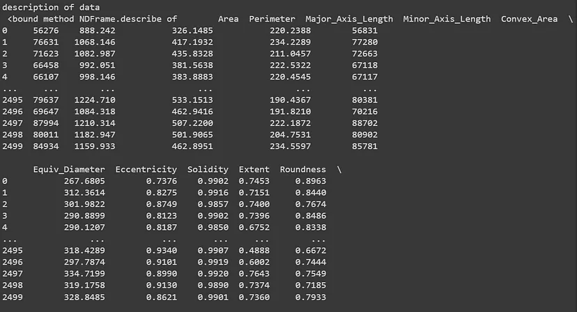
In the data we have, we have 13 columns from which we have one target data and 12 independent variables. Let’s check the description of the data.
print(‘description of data n’, data.describe)
Output:
Let’s check for the null values in the data.
print(‘Null values in data n’,data.isnull().sum(
Output:
There is zero null values in the data so we don’t need to worry about null value analysis.
print(‘datatype in data n’, data.info(
Output:
Here we can see that all independent variables are either in integer format or in float format. Checking the target variable distribution in the data.
data[‘Class’].value_counts().plot(kind = ‘pie’)
Output:
The data we have can be considered a balanced dataset because the number of data points for both classes is almost similar.
Checking the distribution of the Area variable against both classes of pumpkin seeds.
fig_size = (15,8)
plt.figure(figsize=fig_size)
sns.histplot(data = data , x = ‘Area’,hue = ‘Class’,multiple=’dodge’).set(title = ‘Area Distribution’)
plt.show()
Output:
Here is the distribution of the area of pumpkin seeds, by looking at the above visualization we can say that the highest peak of area for both seeds is not equal, which represents a basic difference between the area of both types of seeds.
The area of Çerçevelikseeds is higher than the Ürgüp Sivrisi seeds. Similar observations can be made for all the variables. Let’s take a look:
Perimeter Distribution
fig_size = (15,8)
plt.figure(figsize=fig_size)
sns.histplot(data = data , x = ‘Perimeter’,hue = ‘Class’,multiple=’dodge’).set(title = ‘Perimeter Distribution’)
plt.show()
Output:
It was obvious that the results will be the same as for the Area distribution. Let’s check for the distribution of the major and minor axis lengths.
fig_size = (15,8)
plt.figure(figsize=fig_size)
plt.subplot(1, 2, 1)
sns.histplot(data = data , x = ‘Major_Axis_Length’,hue = ‘Class’,multiple=’dodge’).set(title = ‘Major Axis Distribution’)
plt.subplot(1, 2, 2)
sns.histplot(data = data , x = ‘Minor_Axis_Length’,hue = ‘Class’,multiple=’dodge’).set(title = ‘Minor Axis Distribution’)
plt.show()
Output:
Again the observation is the same that the length of both axes, where Çerçevelikseeds axis lengths are higher. Now we can draw the same plot for the convex areas.
fig_size = (15,8)
plt.figure(figsize=fig_size)
sns.histplot(data = data , x = ‘Convex_Area’,hue = ‘Class’,multiple=’dodge’).set(title = ‘Convex Area Distribution’)
plt.show()
Output:
let’s draw the distribution of eccentricity, solidity, extent and roundness.
fig_size = (15,8)
plt.figure(figsize=fig_size)
plt.subplot(2, 2, 1)
sns.histplot(data = data , x = ‘Eccentricity’,hue = ‘Class’,multiple=’dodge’).set(title = ‘Eccentricity Distribution’)
plt.subplot(2, 2, 2)
sns.histplot(data = data , x = ‘Solidity’,hue = ‘Class’,multiple=’dodge’).set(title = ‘Solidity Distribution’)
plt.subplot(2, 2, 3)
sns.histplot(data = data , x = ‘Extent’,hue = ‘Class’,multiple=’dodge’).set(title = ‘Extent Distribution’)
plt.subplot(2, 2, 4)
sns.histplot(data = data , x = ‘Roundness’,hue = ‘Class’,multiple=’dodge’).set(title = ‘Roundness’)
plt.tight_layout()
plt.show()
Output:
Now the observations are changed because eccentricity and solidity distributions are higher for the Ürgüp Sivrisi seeds and the remaining are similar to the others apart from eccentricity and solidity distributions.
fig_size = (15,8)
plt.figure(figsize=fig_size)
plt.subplot(1, 2, 1)
sns.histplot(data = data , x = ‘Aspect_Ration’,hue = ‘Class’,multiple=’dodge’).set(title = ‘Aspect Ration Distribution’)
plt.subplot(1, 2, 2)
sns.histplot(data = data , x = ‘Compactness’,hue = ‘Class’,multiple=’dodge’).set(title = ‘Compactness Distribution’)
plt.show()
Output:
Here again, aspect ratio and compactness distributions are higher for the Çerçevelik seeds. Let’s move toward the correlation analysis.
However, with decision tree algorithms, we don’t need to perform correlation analysis; to understand the data, we need to do so.
fig = px.imshow(data.corr(
fig.show()
Output:
The above plot represents how the continuous values are correlated to each other but the visualization is not clear here. So let’s drop some lower correlation values.
corr = data.corr().abs()
kot = corr[corr>=.5]
plt.figure(figsize=(12,8
fig = px.imshow(corr[corr>=.5])
fig.show()
Output:
Here we can easily see the highly correlated values. Looking at the graph, we can say how two variables are highly correlated. For example, Area and convex Area are correlated. Now, it’s sufficient data analysis to understand the data, and we can move toward our next step.
Data Preprocessing
Since the data is not so difficult, we can take only two sub-steps to complete this step:
Label encoding
Data Splitting
Label Encoding: in this, we will label encode our class variables using the LabelEncoder function of sklearn in the following way:
Here we can see that class labels are converted into integer format.
Data splitting: here we will split the data into two subsets for training and testing purposes. Using the train_test_split we will split this data into a 70:30 ratio.
from sklearn.model_selection import train_test_split
Here our dataset is split into two subsets. Let’s move toward the next move.
Modelling
Training
In the above, we have made a train and test set of the data and here we are required to fit a decision tree model on the train data. This can be completed using the below lines of codes:
from sklearn.tree import DecisionTreeClassifier
clf = DecisionTreeClassifier(random_state=42)
clf.fit(X_train, y_train)
Lets plot the tree using which the clf object has learnt.
We will need to zoom in on this plot to understand how the data set is split into root nodes and other nodes. The model we used is a simple decision tree model that has taken the aspect ratio as its root node. Let’s check the performance of the model.
pred = clf.predict(X_test)
from sklearn.metrics import classification_report, f1_score, precision_score, recall_score, confusion_matrix
Here we can see without any modification on the base model, the model has performed well, which we can understand by seeing the accuracy, confusion matrix and F1 score.
Let’s try to improve the model’s performance using a grid search approach where we are required to give a set of model parameters. This approach will use all possible combinations of the model and will tell the best fit set of parameters for the model.
params = {
‘max_depth’: [2, 3, 5, 10, 20],
‘min_samples_leaf’: [5, 10, 20, 50, 100],
‘criterion’: [“gini”, “entropy”]
}
from sklearn.model_selection import GridSearchCV
grid_search = GridSearchCV(estimator=clf,
param_grid=params,
cv=4, n_jobs=-1, verbose=1, scoring = “accuracy”)
grid_search.fit(X_train, y_train)
Output:
Here, we can see that we have fit 200 possible models. Let’s take a look at the scores of all the models.
score_df = pd.DataFrame(grid_search.cv_results_)
print(score_df.head(
Output:
Here we can see some results of the grid search approach. Using this data, we can select any of the models but here we will use only the best-fit set of parameters to fit the model. Using the below code we can do so.
grid_search.best_estimator_
Output:
Here, we get the values of the best fit model according to the grid search approach. Now let’s make a model using these parameters.
After zooming in on the plot we can see that this time decision tee has considered the compactness of the seed as its root node. let’s check how the performance of the model has increased this time.
Here we can clearly see that our model’s accuracy and F1 score has increased by 4% and there is more correction in the confusion matrix.
Final word
In this article, we looked at an example of working with a decision tree model to see how we can classify pumpkin seeds into two categories using different parameters of seeds. With this, we have performed the EDA step to understand the data. Decision tree algorithms are one of the most used algorithms in real-life use cases, and also a base model for many high-level models like the random forest, XGboost etc., so it helps understand many high-level models.
You can find our other articles in this link, where we talk about different algorithms, trends and uses of data science and artificial intelligence in real life. The code link, data link and reference articles links are given below for reference.
Data Science Wizards (DSW) is an Artificial Intelligence and Data Science start-up that primarily offers platforms, solutions, and services for making use of data as a strategy through AI and data analytics solutions and consulting services to help enterprises in data-driven decisions.
DSW’s flagship platform UnifyAI is an end-to-end AI-enabled platform for enterprise customers to build, deploy, manage, and publish their AI models. UnifyAI helps you to build your business use case by leveraging AI capabilities and improving analytics outcomes.
Data distribution plays a major role in defining a mathematical function that can help in calculating the probability of any observation from the data space. There are various uses of data distribution we find in the statistical and data science processes. For example it can describe the grouping of observations in a dataset. This is one of the major statistics topics and helps understand the data better. In this article, we will discuss the statistical data distribution basics using the following points.
Table of Contents
What is distribution?
What is density Function?
Types of Distribution in Statistics
Gaussian Distribution
Student T-distribution
Chi-squared Distribution
Bernouli Distribution
Binomial Distribution
Poisson Distribution
Exponential Distribution
Gamma Distribution
What is Distribution?
We can think of distribution as a function that can be used to describe the relationship between the data points in their sample space.
We can use a continuous variable like Age to understand this term where the Age of an individual is an observation in the sample space, and 0 to 50 is the extent of the data space. The distribution is a mathematical function that will tell us the relationship of observations of different heights.
Often generated data follows a well-known mathematical function like The Gaussian Distribution. Generally, these functions are capable of fitting the data if the parameters of the functions are modified. The distribution functions can be used to describe and predict related quantities and relationships between domain and observation.
What is Density Function?
The distribution of data points can be described by their density or density function. Using this function, we describe how the proportion of data changes over the range of the distribution. There are mainly two types of density functions:
Probability Density Function: Using this function, we can calculate the likelihood of a given value or observation in its distribution space. Often we summarise this for all observations across the distribution space. While we plot this function, we et shape of distribution as a result. Using the plot, we can tell the type of distribution in the data.
Cumulative Density Function: Using this function, we can calculate the cumulative likelihood of a given value or observation in the sample space. We can get the cumulative density function by adding all prior observations in the sample space In the probability density function. By plotting this function, we can understand how data is distributed before and after a given value. The plot of this function often varies between 0 to 1 for the distribution.
One noticeable thing here is that both of these functions are continuous functions and in the case of discrete data probability mass function is equivalent to the probability distribution function.
Here we get knowledge of distribution and density functions. After that, types of distribution come into the picture. Let’s take a look at different types of distribution.
Types of Distribution
There are mainly three types of distribution:
Gaussian Distribution
This type of distribution is most commonly found distributions in real-world data. That’s why we sometimes call it the normal distribution. This distribution is named after Carl Friedrich Gauss and mainly focuses on the field of statistics.
The following two parameters help in defining the gaussian distribution:
Mean: a Quantity that is an intermediate value of the large distribution of data observations.
Variance: A quantity that helps in measuring the spread between data observations.
To measure the variance, we often use the standard deviation that defines the spread of data observation from their mean values.
Using the below code, we can make data where observations are normally distributed and plotting them gives us a perfect example of normal or gaussian distributed data.
#importing libraries
import numpy as np
import matplotlib.pyplot as plt
from scipy import stats
#making data
array = np.arange(-10,10,0.001)
data = stats.norm.pdf(array, 0.0, 2.0 )
#ploting probablity density function
plt.plot(array, data)
Output:
Here mean of the data is zero, and the standard deviation is two. For the same data, we can also plot the cumulative density function.
CDF = stats.norm.cdf(array, 0.0, 2.0 )
plt.plot(array, CDF)
Output:
As defined in the code here in the plot, we can see that 50% of the data is lying below the mean(0) point.
Student T-distribution
Estimating the mean of a normal distribution with samples of different sizes is the reason behind this distribution. We can also call it t-distribution. Calculation of this distribution is helpful when describing the error in estimating population statistics for data drawn from Gaussian distributions, and the sample size is taken into account.
The degree of freedom can be used to describe the t-distribution. Also, the calculation of the degree of freedom is one of the main reasons behind using the t-distribution. Using the degree of freedom for any observation helps in describing the population quantity.
For example, if the degree of freedom is n, then we can use n observation from the data can be used to calculate the mean of the data.
Two calculate the observation in a t-distribution, we need to know the observations n the gaussian distribution so that we can define the interval for the population mean in the normal distribution. Observations in t-distribution can be calculated using the below formula:
Data = ( X — mean(X)) / S / sqrt(N) )
Where,
X = observations from normal or gaussian distributed data.
S = standard deviation of X.
N = total number of observations
We can calculate and plot the PDF and CDF for this distribution using the following lines of code.
Calculating Probably Density Function
DOF = len(array) — 1
PDF = stats.t.pdf(array, DOF)
plt.plot(array, PDF)
Output:
Calculating Cumulative Density Function
CDF = stats.norm.cdf(array, 0.0, 2.0 )
plt.plot(array, CDF)
Output:
Chi-Squared Distribution
This type of data distribution helps in describing the quantity of uncertainty of data drawn from the Gaussian distribution. One of the best examples of a statistical method is the chi-squared test, where chi-squared distribution is used often. This distribution can also be used in the derivation of the t-distribution. Like t-distribution, this can also be described using the degree of freedom of observation.
Observation in this distribution can be calculated as the sum of k-squared observations drawn using the Gaussian distribution. Mathematically,
Where,
Z1, …, Zk are samples that are gaussian distributed, and with the degree of freedom k, we can denote chi-squared distribution as
Again, like t-distribution, data usually do not follow this distribution here. Instead, observations are drawn from chi-squared distribution in statistical method calculation for a part of gaussian distributed data.
We can calculate and plot the PDF and CDF for this distribution using the following lines of code.
array = np.arange(0,50,0.1)
DOF = 10
PDF = stats.chi2.pdf(array,DOF)
plt.plot(array,PDF)
Output:
Here we can see that as given the degree of freedom, the distribution changes because the sum of the square random observations from the normally distributed data is under the degree of freedom(10 in this case). However, it is bell-curved but not symmetric.
Calculating the cumulative density function:
CDF = stats.chi2.cdf(array,DOF)
plt.plot(array,CDF)
Output:
Here we can see that there is a fat tail at the right of the distribution, which is continued to the last point.
Bernouli distribution
This type of data distribution mainly comes into the picture when there are only two possible outcomes, and this distribution describes the probability of an event that has been reported only once.
The example of outcomes can be success and failure, 0 and 1, yes or no. to describe this distribution, we use only one parameter, which is the probability of success. Using the below lines of code, we can create a situation with Bernoulli distribution.
We can simply consider the above example as a result of a coin flip, where we can consider any side as a success, and the probability of success will be 0.5.
Binomial distribution
The above distribution was repeated only once but this type of distribution models the number of successes in a situation of repeated Bernoulli experiment. This directly focuses on a success count instead of focusing on the probability of success.
As discussed above, this distribution can be described using two parameters:
Number of experiments
Probability of success
We can use the below line of codes to take an idea of the binomial distribution.
We can compare the above example with flipping a coin ten times, and the graph gives us the probability for each number of success out of 10.
Poisson Distribution
This distribution includes the time parameter with it. Till now, we have seen distribution for one event and a number of events, but here this distribution describes the number of events in a time period. A simple example of this type of case is the number of vehicles passing through a toll booth in 1 hour.
In the extension of the example, we can say there is an average value of vehicles passing through toll booths for different units of time. To describe this distribution, we only need the time parameter. Let’s take a look at the below codes:
The example can be compared to a toll booth where, every one-hour time interval, a number of cars are passing.
Exponential distribution
From the above distribution, if we replace the event per unit time with the waiting time between events, we get the exponential distribution. Simple by inversing the time parameter in the Poisson distribution, we can get describe this distribution.
Here we need to read the x-axis as the percentage of unit time. Here we have 4 events to take place in one hour.
Gamma distribution
This type of distribution can be described by the wait time for an event to occur. We can think of it as a variation of exponential distribution because it takes parameters for the number of events to wait for with the lambda parameter of the exponential distribution.
We can take an example from the bus that is waiting to run when the number of passengers is not filled in it. Let’s take a look at the below graph.
time = 4 # event rate of customers coming in per unit time
In the above graph, we can see that the peak is around 2.5, which means the waiting time for ten passengers to come on the bus is 2.5 times the unit time of 2 minutes.
Final words
In this article, we have discussed data distribution, Density Functions and Type of Distribution in data. In statistical and data science processes, these all things come in the early stages of processes that helps us in generating more knowledge about the data we have. Since understanding the data domain and statistics are important tasks for a data scientist, with the help of the above-given knowledge, we can understand the statistics of our data.
Data Science Wizards (DSW) is an Artificial Intelligence and Data Science start-up that primarily offers platforms, solutions, and services for making use of data as a strategy through AI and data analytics solutions and consulting services to help enterprises in data-driven decisions.
DSW’s flagship platform UnifyAI is an end-to-end AI-enabled platform for enterprise customers to build, deploy, manage, and publish their AI models. UnifyAI helps you to build your business use case by leveraging AI capabilities and improving analytics outcomes.
According to a united nation report, the human population of the world is projected to reach 9.8 billion by 2050, and there is approximately 8.0 billion people in 2022. The statistics show that there will be approximately a 20% hike in the human population. One main domain on which human life depends is agriculture, and to complete this gap between the population of today and of 2050, this domain will be required to increase its productivity by 60%. In India alone, growing, processing and distributing food is a 71,220 Billion business.
By looking at today’s scenario, machine learning, data science, and artificial intelligence are potential ways to fulfil the anticipated food needs of people joining us by 2050. As we know that the whole agriculture process is a combination of many other processes, these sub-processes require tracking and monitoring for so long where the size of the farming area is often hundreds of acres, and at the same time, insights like weather, seasonal sunlight and attacking patterns of animal birds, insects are always required to be better modelled. There is plenty of such information that needs to be managed simultaneously, and here machine learning finds itself as a perfect solution to the problem of managing a large size of information at the same time.
The above-given information is why farmers, co-ops and agricultural companies are largely interested in investing in AI. According to a BI Intelligence research report, global spending in agriculture industries on AI and machine learning is projected to reach about $4 billion, which was $1 in 2020. These numbers represent how data-centric approaches are expanding their ways of being applied in the field. The following are use cases AI finds in agriculture.
AI and Machine Learning-Based Surveillance Systems
Applying AI and machine learning models in crop surveillance systems enable farmers to monitor crop fields in real-time and easily identify the animal and human breaches. This way, AI and Machine learning help reduce the chances of the crop being destroyed. These systems record video and give rapid responses based on video analytics. These AI-enabled solutions can be scaled from small farmers to large-scale agriculture operations.
Crop Yield Prediction
Applying surveillance systems on fields can also be used for collecting data, and this helps ML algorithms to analyse real-time video streaming. Also, thanks a lot to IoT(Internet of Things) that helps collect the in-ground data of moisture, fertiliser and natural nutrient levels.
Combining both data AI and ML helps analyse each crop’s patterns over time, as machine learning is a perfect way to combine massive data sets and provide constraint-based advice about crop yield. Also, more advanced level Ai enabled systems can help farmers to improve crop health.
Crop Planning
Yield mapping is a term that involves agriculture and machine learning algorithms together. In-depth, we can say that supervised machine learning models help to find patterns in large agricultural datasets. This helps in understanding the orthogonality of crops in real-time. All these things play a crucial role in crop planning.
With the help of machine learning, it becomes easy to quantify the potential yield rates of a field even before the vegetation is started. To make such predictions, algorithms use social condition data from the in-groud sensor and surveillance-based data of soil colour and atmosphere and help the agricultural specialist to predict soil yields for a given crop.
Pest Management
A former or agricultural organisation can improve pest management by combining surveillance data and in-ground sensor data. International agencies use infrared camera data from drones and in-ground sensor data to monitor crop health and leverage AI to predict pest infestations.
Robots
Various AI and ML-based smart tractors, agribots and other tools help formers to recover the shortage of agricultural workers. These tools and devices are a viable option for many remote agricultural operations. These devices came out as a blessing for large-scale agriculture businesses that not only reduces the cost of employees but also gives higher accuracy in repetitive tasks.
Supply Chain Management
Just like in other supply chain management systems, AI has accelerated the track and traceability across all agricultural supply chains. More impact of this can be seen in the pandemic times. AI and ML models are not only accelerating apply chains but also helping in inventory management where they can easily differentiate between the inbound and outbound shipments’ batch, lot and container level assignments of crops and material.
In a more advanced system, sensors are used to differentiate between the shipment’s and material’s condition.
Pesticides Optimisation
Machine learning models are being utilised to find out the right mix of pesticides and their application in a specified field area. Utilising such models, formers are not only finding the right fit of pesticides but also reducing costs. Using the sensor data and visual data from drone models can detect and segregate defective areas into different classes. Also, these models can tell the right mixes of pesticides for different defective areas.
Final words
Here in the above, we have seen some of the most common use cases of AI and Ml in the agriculture domain. Instead of these, machine learning and AI can also be used to predict the market price of different crops based on the crop yield rate and help us optimise irrigation systems.
When talking about the agriculture domain, we at DSW | Data Science Wizards find endless opportunities for AI and machine learning in the domain that can make it more advanced. Our flagship AI platform UnifyAI has the capabilities of solving AI and ML use cases of any domain in an optimised and accurate way and in reduced timing. We understand that a larger part of the Earth is dependent on agricultural businesses, so it becomes more important to resolve AI use cases in this sector with higher accuracy. Using UnifyAI, we make sure that AI and ML play an important role in advancing our client’s agricultural businesses and helping them to perform easy and effective farming with lesser effort.
About DSW
Data Science Wizards (DSW) is an Artificial Intelligence and Data Science start-up that primarily offers platforms, solutions, and services for making use of data as a strategy through AI and data analytics solutions and consulting services to help enterprises in data-driven decisions.
DSW’s flagship platform UnifyAI is an end-to-end AI-enabled platform for enterprise customers to build, deploy, manage, and publish their AI models. UnifyAI helps you to build your business use case by leveraging AI capabilities and improving analytics outcomes.
In one of our articles, we have already discussed basic concepts hidden behind the decision trees, including the definitions of the decision trees, other core concepts and terminology we use with the algorithm.
As we have already discussed all the theoretical parts of the decision tree, we now need to understand how we can use this model practically. This article will be an extension of the above-given article, where we will discuss the implementation of a decision tree using the python and R programming languages. This article will cover the following topics:
Table of Contents
Implementation of Decision Tree using the Python Programming Language
Data splitting
Importing and Fitting the Decision Tree Model
Model Evaluation
Implementation of Decision Tree using the R Programming Language
Data splitting
Importing and Fitting the Decision Tree Model
Model Evaluation
Implementation of a decision tree using the python programming language
To complete this motive of ours, we will take the help of the sklearn python library that will not only help us in fitting the model on data but also help in importing the iris data.
With the iris data, we get the four continuous variables that include sepal length, sepal width, petal length, and petal width of the iris flowers and based on these variables or features of the data. Iris flowers are separated into three categories: Iris Setosa, Iris Versicolour, and Iris Virginica. Let’s import the data sets.
from sklearn import datasets
data = datasets.load_iris()
X = data.data
y = data.target
print(‘independent variables name n’, data.feature_names)
print(‘shape of independent variables n’, X.shape)
print(‘class names in target variables n’,data.target_names)
print(‘shape of target variables n’, y.shape)
Output:
In the data, we get 150 data points and four variables as discussed above.
Now to model this data using a decision tree, we will use the following steps:
Data splitting
Importing and fitting the decision tree model
Model evaluation
Let’s start with data splitting.
Data splitting
This step makes two sets of data ( train and test). Using the train set, we will train a decision tree mode and using the test set, we will evaluate the trained model. Let’s split the data.
from sklearn.model_selection import train_test_split
X_train, X_test, y_train, y_test = train_test_split(X, y, random_state = 0)
Let’s check the shape of the spilted sets
print(“shape of train data”, X_train.shape, y_train.shape)
print(“shape of test data”, X_test.shape, y_test.shape)
Output:
Importing and Fitting the Decision Tree Model
This step will let us know how to fit the decision tree model on data. The point to be noticed here is that the model from sklearn takes a NumPy array form of data to train the model. Also, calling the data from the sklearn library comes as a NumPy array, so here we are not required to worry about any transformation. We can directly fit the split data. Let’s import and train the model.
Here we can see that the in the root node of the decision tree, if the value of petal width is below or equal to 0.8, then iris has a class, and there are 37 samples of such data in whole train data. If the petal width is larger than 0.8 cm, then the iris flower is of a different class.
Let’s make predictions using the test data.
prediction = clf.predict(X_test)
Here in the prediction variable, we have values predicted by the model for the test data. Now, we can evaluate our model using the prediction set against the true values.
Model Evaluation
This section will use the accuracy score, f1_score and confusion matrix to evaluate the model. But, first, their definition is explained below.
Accuracy score: This gives the results based on the calculation of how many right predictions are made by the model compared to real data.
F1_score: This gives the harmonic mean of the precision and recall. Where precision can be interpreted as the right predicted positive values that belong to the positive class, and recall can be interpreted as the number of positive predicted values made out of all positive examples in the dataset. Mathematically,
print(‘accuracy score of our model n’, accuracy_score(y_test, prediction
print(‘f1 score of our model n’,f1_score(y_test, prediction, average = ‘micro’
Output:
Here we can see that there is only one value that the model has predicted wrong, and it has achieved a 97 % accuracy with a similar f1_score. Here this implementation is completed, and in the next section, we will perform the same operations using the R programming language.
Implementation of a Decision Tree using the R programming language
To work with the same data in the R programming language, we can use the datasets library. Using the below codes, we can get the Iris data.
ibrary(datasets)
data(iris)
head(iris)
Output:
Here we can see what how exactly our data looks like. Now we will follow the same steps as we followed using the Python programming language.
Data splitting
To complete this step, we will use the caTools library.
Here we have split the data into an 80/20 ratio, where 80% of the data is from training, and 20% is for testing the model.
Importing and Fitting the Decision Tree Model
To complete this step, we will use the rpart library that allows us to fit the decision tree to any data. Using the below codes, we can call and train the model.
library(rpart)
clf <- rpart(formula = Species ~., data = train_data,
method = “class”,
control = rpart.control(cp = 0),
parms = list(split = “information”
Let’s check the model by plotting it.
library(rpart.plot)
prp(clf, extra = 1, faclen=0, nn = T,
box.col=c(“green”, “red”
Output:
One thing which we can also do here is to use the caret library so that we can check the importance of the feature/variable of our data in data modelling.
library(caret)
importances <- varImp(clf)
importances
Output:
Here we can see that the petal width is the most important variable in the training of the decision tree model.
Let’s make predictions from the model.
prediction <- predict(clf, newdata = test_data, type = “class”)
prediction
Output:
This is how our model has predicted on the test data.
Model Evaluation
Using only one line of codes we can evaluate our model against various matrices.
confusionMatrix(test_data$Species, prediction)
Output:
Here we have got most of the statistics which can be utilised to evaluate the model and we can also see that model has predicted only 1 wrong values and the accuracy of the model is around 97%.
Final words
The decision tree can be interpreted as an excellent introductory model to the tree-based model family. We can also find its uses as a common baseline model for various models like random forest and gradient boosting.
This article has looked at how we can implement a decision tree model using the python and R programming languages. With this, we have also looked at how we can draw and evaluate the model. Shortly we are going to cover all such kinds of models and concepts of machine learning and data science. To get all information, you can keep yourself connected to this link.
Data Science Wizards (DSW) is an Artificial Intelligence and Data Science start-up that primarily offers platforms, solutions, and services for making use of data as a strategy through AI and data analytics solutions and consulting services to help enterprises in data-driven decisions.
DSW’s flagship platform UnifyAI is an end-to-end AI-enabled platform for enterprise customers to build, deploy, manage, and publish their AI models. UnifyAI helps you to build your business use case by leveraging AI capabilities and improving analytics outcomes.
In 1983, the idea of open source technology came out as a revolutionary step in the software development field, where Richard Stallman found this ideological movement of making source codes of the software accessible to programmers. From 1983 to now, we can witness 180,000 open-source projects available and 1400 unique licences available to handle these projects.
It is found that open source technologies provided many opportunities, an extensive amount of innovations and stability to the software development field. In this article, we will discuss how these technologies provided so many changes in the sector using the following points:
Table of Contents
What is Open Source Software?
Need for Open Source Software
How does Open Source Software work?
Examples of Open Source
What is Open Source Software?
When the source codes of any software are accessible to everyone for inspecting, modifying and enhancing, the software is called open source software(OSS).
In traditional ways, these source codes were a part of the software that most computer users couldn’t see. When we talk about source codes of any software, we can say that they are the building block of any software and can be manipulated by computer programmers. The changes performed by programmers are intended to make changes to the program or application of the software.
When it comes to the protection of open source software and communities, the open source initiatives(OSI) come into the picture that acts as a governing and central information repository of open source software. The OSI comes with guides and rules that decide the use and interaction with OSS and includes support and community information, and definitions to help users understand and treat OSS ethically.
Need for Open Source Software
Various reasons make OSS important in today’s scenarios. Some of them are as follows:
Control: Control of any software is one of the important requirements nowadays, and people want to know how the building blocks and source codes are designed to perform any task. So if they find something not required or needs some changes, they can accomplish it by themselves instead of using a standard for all versions of software.
Innovation: one major reason behind the success of OSS is it allows people to come and perform practicals on the source codes so that they can either use the OSS efficiently or study and learn from the codes. This learning directly leads to more innovative approaches to programming also, as people can improve OSS, which is beneficial for the OSS communities.
Stability: many users find that a well-managed OSS are more stable than closed source software. The forums and community pages of an OSS help it keep track of bugs and improvements. Also, people from outside management and the development team can handle these bug fixes and improvements.
Security: Many consider OSS more secure than closed-source software in their workflow. Since many programmers can work together to resolve the unspotted errors by the author, it becomes a more feasible and quickest way to solve them.
How does Open Source Software work?
As described above, source codes of OSS are available to everyone, which means they are stored in a public repository so one can use them independently. Instead of just using them, one can also perform code changes so that OSS’s design and functionality can improve.
In case of source code changes taking place, OSS requires recording and maintaining those changes, including the method of performing changes.
Examples of Open Source
The Internet is one of the best examples of open source, where most of the fundamental function we find on the Internet is built in the open source environment. For example, Linux OS helps regulate the web server’s operation and the apache web server application, help data transfer between the personal devices and world wide web infrastructure or vice versa. As given above, there are countless applications and software that are open source.
We can also witness that large internet companies like Facebook and Google have made their various software open-sourced to benefit from more innovations and enhanced stability.
Now we know open source development welcomes innovation through collaboration and is a reason behind many different and new technology that meet us instead of taking them for granted. Because of open source involvement, we can see the breakneck speed of software development.
Final words
This article discusses the meaning, requirement, and working of open source software(OSS) and the difference between open source software. Because of this discussion, we get to know that making any software or project open-sourced opens many doors for development and improvement. Also, this step moves us towards social causes because it not only helps many programmers to learn and innovate but also pushes them to see how these projects work in resolving real-life use cases.
We admire this approach because it showcases a desire to share and transparently collaborate with others. Using this technology, we find ourselves playing an important and active role in developing a better world because everyone is contributing to us and helping us impact areas like finance, retail, health, education, and manufacturing using open source values.
In today’s scenario, artificial intelligence is becoming a mandatory part of every domain and industry. Particularly in the Retail domain, we can witness digital transformation advancing the sector for years. Implementing AI-based systems in retail has increased the number of use cases, development speed, efficiency, and accuracy. At the same time, advanced data and predictive analytics models are helping the domain to make smart, data-driven business decisions and future predictions to understand the specific needs of customers.
Thanks to the internet of things(IoT) that helps in generating or gathering more data and increases the opportunity of applying AI in retail industries. Artificial intelligence is a domain that understands the value of every data and can be leveraged to improve operations and new business opportunities. Moreover, a fortune Business Insights report says that the global artificial intelligence in the retail domain is projected to grow up to USD 31.18 Billion by 2018 at a CAGR of 30.5%.
The above statistics represent the competitive environment between the retail businesses, and everyone in the industry will not risk losing their invincible market share to their competitors. So let’s start understanding why AI can make this domain more advanced.
How does AI take Part in the Retail Business?
Undoubtedly, artificial intelligence has found its way into many industries. However, many people don’t understand its meaning. Applying AI to any industry means applying various technologies like machine learning, predictive analytics, and robotics. The main motive of implementation is collecting and processing data and using it to predict, classify and reduce human mistakes so that the industry can work fluently and accurately and humans are able to make data-driven decisions.
When we look back at the recent history of retail businesses, we find that the digital transformation of the industry has started with applying primary IoT devices that are basically data sources. Nowadays, AI is in front of us as advanced technology, and as it finds data in any industry, it finds its use cases. Things have changed a lot in recent scenarios because we can find that giants like Amazon and Reliance are applying behaviour analytics and customer intelligence to extract valuable insights so that touchpoints in the customer service sector can also be improved. Behaviour analytics and customer intelligence are a part of artificial intelligence systems.
What are the advancements?
Nowadays, retail industries are built on top of AI, data-driven decisions and experiences and higher customer expectations. Using AI, we can deliver personalised shopping experiences at scale, which is more relevant and valuable. A simple example of change from traditional retail business is that digital and physical purchasing channels are blended, which helps retailers make their retail channels more advanced and think on the innovation side. As a result, such retailers distinguish themselves from others to become market leaders.
Here are some examples or subdomains of the retail industry where AI plays an important role:
Inventory management
As discussed above, AI is being used to generate a forecast of demand. This use case can be resolved using mined insights of the marketplace, consumer and competitor data. Using the demand forecast, retailers can understand the industry shift and accordingly perform changes in the marketing, merchandise and business strategies.
Adaptive Webpages
Pages of mobile or computer applications can recognise the customers and their shopping patterns even in real-time. That is why we can witness that they are presenting information and product based on our current, previous purchases and shopping behaviour. Also, such systems are designed to evolve constantly so that information can be hyper-relevant to every customer’s marketing and purchasing behaviour.
Dynamic Recommendations
Recommendation systems are also a part of AI that deals with a lot of data analysis and machine learning combining. They can be designed as they can learn and store customer behaviour and preferences through customers’ repetitive interaction or purchasing. All information is saved as a proper profile and utilised for delivering proactive and personalised outbound marketing.
Interactive Chatbots
We can think of this use case of AI as a standard use case for every domain because chatbots are very helpful in improving customer service and engagement. For example, in retail, these bots help retailers to communicate with their customers using the power of AI and machine learning. Trained chatbots can help answer common customer questions and directs them to beneficial outcomes. In turn, these chatbots become more valuable when collecting a customer base that directly leads retailers to make future business decisions.
Visual-based Curation
As we know that there are various algorithms that can translate image, particularly saying image-to-text algorithms helps retailers to represent their new or related products using image-based search or old customer behaviour. Nowadays, these AI-based models can curate recommendations for customers based on aesthetics and similarity.
Guidance in Discovery
In every retail platform, there s always a need to provide confidence to the customer in their purchasing. AI assistance can help narrow down the selection and provide recommendations based on the requirements like preferences and fitting.
Customer insights and personalisation
AI-enabled personalisation systems can recognise the customers and reflect their profile and loyalty to the retailers; based on that, customers can be classified, and some perks like price variations and rewards can be given to them.
Using the stored data AI can tell us what a customer might be interested in using customers’ demographics, social media behaviour, and purchasing patterns. These use cases can work for both online and offline shopping platforms.
Operational Optimisation
Various AI systems help retailer manage their inventory, staffing, product, and delivery systems, even in real-time. Using such systems, retailers create an efficient system or environment that can meet customers’ requirements and expectations immediate and qualitatively high.
Need for AI in the retail industry
In the above points, we have covered some of the major use cases where AI plays an important role in giving solutions in the retail industry.e can understand that digital transformation of the retail industry is a necessity, and also, there are countless benefits of applying AI in this sector. Because this industry is one of the top data-generating industries, there are countless opportunities for AI in the future.
We at DSW | data science wizards have extensive experience in working with retail industry clients. Because of this, we understand the values and business that AI can add to this sector. Here are five primary benefits of AI that retailers can count on.
Captivate Customers –
A huge number of retail businesses provide immersive shopping experiences to the customers, and here traditional retailers require more customer engagement, and AI is a way to help them in a more personalised and relevant manner.
Satisfactory Customer Experience
Every retailer can understand the value of customers’ interests. Offering consumers compelling services and experiences is a touchpoint where retailers can differentiate from others. Predictive analytics is a domain of AI that helps retailers to make a difference. A retailer can lead with such innovation rather than just following the traditional way and reacting to the recent changes.
Finding More Data Insights
There is a huge rush of information in the retail sector. Here retailers need to filter out the important information and transform that into customer-first strategies.
Blending Offline and Online Retail
Treating offline and online different from each other can be a huge mistake for retailers. Nowadays, these two channels are no more distinct and require a blended way of treatment and operations so that businesses can lead to operational efficiencies from inefficiencies.
Flexible Logistic Networking
A broad range of customer demands fails the traditional supply chain systems and forces retailers to adapt their supply chain to AI and make a flexible ecosystem that can easily and quickly respond to huge demands and customers’ shifting behaviours.
Making a fully AI-enabled retail system seem overwhelming, but it should not have been. We at DSW aim to make AI available for everyone and create an AI-enabled environment that can be leveraged by any domain. Our flagship platform UnifyAI is made with such capabilities that every industry and sub-industry can utilise it to build a data and use-case-centric system to make data-driven decisions. Click here to check out the similar use cases of AI in different domains or industries.
In today’s scenarios, it has become a requirement for organisations to apply such an atmosphere in their data sources so that every piece of information can be utilised efficiently. When using the data for various purposes, we should always remember that the data pipeline is one of the major tools required in the process. As many say, “data is new fuel” data pipeline becomes comparable to fuel pipelines. The data pipeline is an important topic, and using this article, we will learn the following things about it.
Table of Content
What is Data Pipeline?
How does the data pipeline work?
Components of Data Pipeline
Why Data Pipelines are important?
Modern data pipelines and ETL
Future Improvements Needed
What is Data Pipeline?
A data pipeline can be defined as a set of tools and processes used to manage, move and transform data between two or many systems(source and destination). The motive behind applying data pipelines is to cope with every data or piece of information we get or generate. In simpler terms, we can say a data pipeline is a way that starts by collecting data from various sources and ends at a destination where data is being used to generate profits of data. Still, in between the way, multiple processes increase the usability of data at the destination source.
How does the data pipeline work?
As the above defined, it is simple to understand that the work of a data pipeline is to collect the data from different sources and take it to the destination source, where further processes like data analysis and predictive modelling work on the data. The data processing along the way depends on the requirement of use cases. However, using the data pipeline, we focus more on managing data in a more appropriate or advanced manner.
A simple example of handling data is preparing data for a machine learning program where a machine learning program is a destination, and data silos are the source. Data silos can hold all the data of an organisation and when applying machine learning for any use case organisation needs to push only a few or required data in training instead of pushing all data from data silos. In such a situation, a data pipeline takes required-raw data from silos(source) and pre-processes it along the way(null value identification, numeric transformation, dimensionality reduction etc.) and serves the data to machine learning algorithms.
Components of Data Pipeline
Using the above-given example, we can say such data pipelines will require the following components:
Data Sources: Data sources can be of various types, such as relational databases and data from applications. Often we see that pipelines take raw data from various sources using a push mechanism, API call, and replication engine. These all together pull or supply data continuously or a webhook. Also, there may be data being synchronised in real-time or at scheduled intervals, which takes extra effort to manage data in the source.
Data collection: This component is responsible for collecting important data into the data pipeline. Such components carry data ingestion tools so that various data sources can be connected together.
Transformation block: The transformation of data is a must process to get completed along the way of pipelines that can include sorting, deduplication, validation, and standardisation of the data. The motive behind applying this block is to make data analysable.
Processor: Machine learning models can ingest data in two ways. Whether in batches or in streamline. In batch processing, we collect data for predefined time intervals, and in the streamline, we process and send data to the model as data is generated.
Workflow: This block helps in the sequencing and management of dependency. Used dependencies can be business or technical-oriented.
Monitor: Data pipelines compulsorily have data monitoring systems so that we can get ensure data integrity. Network congestion of offline sources or destinations can be an example of a potential failure situation that can be prevented by applying alerts for such scenarios.
Destination source: A destination source is one step before the machine learning algorithms and examples of it can be on-premises databases, cloud-based databases, or data lakes. It can also be an analytical tool like Power BI, and tableau.
The below image can be a representation of the data pipeline.
Why Data Pipelines are important?
As we all know, most organisations generate data from more than one source, and since all the data gets collected in one place, lake, or silos, it becomes complex to fetch valuable data from such complex storage. Moreover, various processes require data in time, and they really matter for an organisation’s growth, like business intelligence processes where tracking day-to-day life requires information or data every day. Avoiding mistakes in accessing and analysing data pipelines is very important.
Since organisations are requiring real-time analytics to make faster, data-driven decisions. The data pipeline eliminates the manual and time-taking steps and events from the process and enables a smooth, automated flow of data throughout the different data sources
In some places, consistent data quality is one of the major concerns and data pipelines are very helpful in ensuring the required data quality because it includes transformation and monitoring processes in it.
Modern data pipelines and ETL
Generally, ETL tools work with the data warehouses(in-house) and help in extracting, transforming and loading the data of different sources. In more recent scenarios there are various cloud data warehouse services like Google BigQuery, Amazon Redshift, Azure and Snowflake available. These warehouses are capable scale up and down the processes in seconds or minutes which helps developers in replicating raw data from disparate sources in SQL. After that, they can define transformation procedures for data and run them through the data warehouse after loading.
Also, there are various cloud-native warehouses and ETL services for the cloud are available. Using such options organisations can set up a cloud-first platform and data engineers are required to monitor ad handle failure points or unusual errors.
Future Improvements Needed
In recent scenarios, we can witness the boom in the fields of Artificial intelligence(AI), data science and machine learning. Looking at these opportunistic fields we can say that in near future every organizations that is generating the data will be using new technologies. Data and only required data is one of the major requirement to make these technology work appropriately.
In the above sections we have scene that data pipelines works and AI-ML models requires few more changes in the data like numeric data, data without null values etc. so as the demand of ML increasing changes in the data pipeline is also increasing. One major change we find is addition of feature store before the model layer. As models are data specific they works with high accuracy when required feature is provided.
Feature store can be explained as the storage system of only those daa points which are usable for the model presented in the next layer. Here we can say that feature store is one improvement and if applied in data pipeline its block diagram will look as following:
At DSW | Data Science Wizards, we have worked with many clients who were requiring AI models to be applied in their workflow and data pipeline. If we look back at our article, we can know how features stores are an essential participant in the data pipeline, especially when the pipeline is ending on an AI-model
We come with our flagship platform UnifyAI and aim to make AI available for everyone.
This platform uses some essential components to build, orchestrate and leverage AI capabilities for use cases across the domains, and the feature store is one of those components. Using Its feature store, this platform helps reduce the time of building and resolving new use cases using AI-enabled solutions.
About DSW
Data Science Wizards (DSW) is an Artificial Intelligence and Data Science start-up that primarily offers platforms, solutions, and services for making use of data as a strategy through AI and data analytics solutions and consulting services to help enterprises in data-driven decisions.
DSW’s flagship platform UnifyAI is an end-to-end AI-enabled platform for enterprise customers to build, deploy, manage, and publish their AI models. UnifyAI helps you to build your business use case by leveraging AI capabilities and improving analytics outcomes.