Blog

In our series of articles, we have provided a comprehensive introduction to time series analysis, covering various aspects such as the components of time series and the necessary steps to perform a thorough analysis. In this particular article, we will focus on an important aspect of time series analysis, which is handling missing values in time series data. This falls under the category of time series preprocessing and data exploration.

Throughout this article, we will explore the significance of imputing missing values in time series data and delve into various methods that can be employed to achieve this. The following table of contents outlines the key topics covered in this article:

Table of Contents

• Importing a Time Series dataset
• Finding Missing Values
• Forward-Filling Method
• Backward-Filling Method
• Linear Interpolation
• Trend and Seasonal Decomposition

Let’s start with importing a time series dataset.

Importing a Time Series Dataset

In this article, we are going to download market data from Yahoo! Finance’s API, for which yfinance’s open source tool is going to help us, which uses Yahoo’s publicly available APIs. Using the following line of code, we can install it in our environment.

!pip install yfinance

After installing this module, we are ready to download the market data of any company for this article, and we will use the reliance company’s market data of last year. Let’s do this.

import yfinance as yf
data = yf.download(“RELIANCE.NS”, start=”2022–01–01″, end=”2023–01–01″)
print(data)

Output:

Here we can see an overview of this data. In this data, we can see that there are 248 rows for 365 days of data, which means there are some missing dates in the data.

When we consider time series analysis as a process, we need to understand that not only missing data values are called missing values in time series but also the missing time values from the sequence of time is called missing value in the data. To learn about handling general missing values from data, we can refer to this article. In this article, we will learn how to handle missing values, specifically in time series data. Let’s move to the next sections and learn how to handle missing values in time series data using different methods.

Finding Missing Values

Before handling the missing values in time series data, it is necessary to find the time values that are missing from the time series. To find missing time data from a time series, we can use the Pandas library functions. Below is a way to store the missing time values in a series object.

import pandas as pd
data.index = pd.to_datetime(data.index)
date_range = pd.date_range(start=”2022–01–01″, end=”2023–01–01″, freq=”D”)
missing_dates = date_range[~date_range.isin(data.index)]
print(missing_dates)

Output:

Here we get a series object which has a length of 118 which means there are 118 missing in our extracted data. Let’s visualise this using the Matplotlib library’s functions and the Close variable of the data.

import matplotlib.pyplot as plt
plt.figure(figsize=(10, 6
plt.bar(missing_dates, [1] * len(missing_dates
plt.title(“Missing Dates”)
plt.xlabel(“Date”)
plt.ylabel(“Count”)
plt.xticks(rotation=45)
plt.show()

Output:

Here, we can see the visualisation of the missing time values in the graph. Now let’s take a look at the visualisation of the missing data with the close variable of the data.

merged_data = data.reindex(date_range)
closing_prices = merged_data[“Close”] missing_dates_mask = closing_prices.isna() # Plotting the closing prices with breaks for missing dates
plt.plot(closing_prices.index, closing_prices) plt.title(“Reliance Closing Prices”)
plt.xlabel(“Date”)
plt.ylabel(“Closing Price”)
plt.grid(True)
if missing_dates_mask[i]:
plt.axvline(closing_prices.index[i], color=”red”, linestyle=” – “)
plt.show()

Output:

Here in the graph, we can see the red lines drawn for the missing dates and the blue lines drawn for close values of the reliance stock price. Now that we know about the missing values in the data, we are ready to apply the missing value handling techniques to it. Let’s start with the forward-filling method of imputing missing values.

Forward-Filling Method

Using this method, we can fill in missing values in a time series using the most recent preceding value. Things to notice here are that in the forward filling, we don’t consider any relationship between the data values, which means this method assumes that the value of the missing data point remains constant until a new value is observed. It is useful when dealing with time series data that exhibits a relatively stable trend or when missing values occur in consecutive intervals. This operation propagates the last observed value forward until encountering the next available data point. Using the below lines of codes, we can perform this with our extracted data.

data_reindexed = data.reindex(date_range)
data_filled_forward = data_reindexed.fillna(method=”ffill”)

Here, we have made the new index of the data using the above-defined date range and applied the ‘ffill’ method to fill the missing dates in the data.

Now we can draw the closing variable and check how the whole data can be presented.

plt.figure(figsize=(10, 6
plt.plot(data_filled_forward.index, data_filled_forward[“Close”], label=”Forward Filled”)
plt.title(“Reliance Closing Prices”)
plt.xlabel(“Date”)
plt.ylabel(“Closing Price”)
plt.legend()
plt.grid(True)
plt.show()

Output:

Here, we can see we have imputed the missing values using the forward-filling method. Now let’s move towards the next method of imputing missing values in time series.

Backward-Filling Method

As the name suggests, we can think of this method as the opposite of the forward-filling method, where we use the most recent succeeding value to impute the missing values in time series data. When applying a backward filling to fill missing values, the next available value after the missing data point replaces the missing value. The backward fill operation propagates the next observed value backwards until encountering the last available data point. Using the below line of codes, we can apply this method to our extracted data.

data_reindexed = data.reindex(date_range)
data_filled_backward = data_reindexed.fillna(method=”bfill”)

Let’s draw the close variable data with respect to the time after imputing with both forward and backward filling so that we can get a comparison between both of the methods as they are similar.

plt.figure(figsize=(10, 6
plt.plot(data_filled_forward.index, data_filled_forward[“Close”], label=”Forward Filled”)
plt.plot(data_filled_backward.index, data_filled_backward[“Close”], label=”Backward Filled”)
plt.title(“Reliance Closing Prices”)
plt.xlabel(“Date”)
plt.ylabel(“Closing Price”)
plt.legend()
plt.grid(True)
plt.show()

Output:

Here, we can see that there is a slit change in both types of data as one is using the most recent preceding value, and on the other hand, the other one is using the most recent succeeding value to impute the missing values in the data. After completion of these two methods, let’s take a look at the other method of handling missing values.

Linear Interpolation

Basically, linear interpolation is a method of estimating values between two known data points. In the context of time series data, we can use linear interpolation to fill in missing values or gaps in the data.

When we go into the deeper side, we find that this process works by creating or assuming a straight line between two adjacent data points and estimating the values at points along that line. To estimate the missing values using this method, we need to consider a linear relationship between the known data points.

We can also consider it as a simple and straightforward way to estimate missing values, especially in cases where the data follows a relatively smooth trend. It is advised not to use this method of imputing data when the underlying relationship is nonlinear or if there are significant fluctuations or irregularities in the data. Like the above-given methods, it is simple to implement; let’s check the below codes.

data_reindexed = data.reindex(date_range)
data_interpolated = data_reindexed.interpolate(method=”linear”)

Here, we can see that we have used the interpolate function given with the pandas’ data frame and specified the linear method to perform the linear interpolation method for imputing missing data in time series data. Let’s take a look at the close variable graph after imputation while comparing it with imputed data using the forward-filling method.

plt.figure(figsize=(10, 6
plt.plot(data.index, data[“Close”], label=”Original Data”)
plt.plot(data_filled_forward.index, data_filled_forward[“Close”], label=”Forward Filled”)
plt.plot(data_interpolated.index, data_interpolated[“Close”], label=”Interpolated Data”)
plt.title(“Reliance Closing Prices”)
plt.xlabel(“Date”)
plt.ylabel(“Closing Price”)
plt.legend()
plt.grid(True)
plt.show()

Output:

Here, we can see the difference between the results from both of the methods, and we can see how assuming a linear relationship between data points worked in imputing the missing value in the data.

Trend and Seasonal Decomposition

In the introduction article, we have already discussed that time series data is a result of several components and trend, seasonality, cycle, and residuals are the four main components of it. By breaking a time series in these components, we can also impute the missing values in time series data.

Since the seasonal component captures recurring patterns or seasonality present in the data

When it comes to imputing missing values in a time series using seasonal decomposition, the approach typically involves the following steps:

• Time series decomposition
• Missing value identification
• Impute Seasonal Component: Here, the seasonal patterns of time series are necessary to take into account, and by this, we can use the average of the corresponding seasonal values from previous and subsequent periods to fill in the missing values.
• Impute Trend Component: If there are still any missing values after imputing the seasonal component, we can fill the rest of the values using the techniques such as linear interpolation or regression-based imputation that estimates the trend component and fill in the missing values accordingly.
• Reconstruct the Time Series.

Let’s take a look at how we can perform this via codes.

Decomposing the time series into its components.

 

from statsmodels.tsa.seasonal import seasonal_decompose
result = seasonal_decompose(data[“Close”], model=”additive”, period=7)

Getting the trend components and filling them using the forward filling method.

trend = result.trend
trend_filled = trend.fillna(method=”ffill”).fillna(method=”bfill”)

Getting the seasonal component and it with the forward filling method.

seasonal_filled = result.seasonal.fillna(method=’bfill’).fillna(method=’ffill’)

Adding components of time series

imputed_data = trend_filled + seasonal_filled + result.resid

Let’s plot the data filled by Interpolation and filled by Trend and Seasonal Decomposition

plt.figure(figsize=(10, 6
plt.plot(data_interpolated.index, data_interpolated[“Close”], label=”Interpolated Data”)
plt.plot(imputed_data.index, trend_filled, label=”Imputed Data”)
plt.title(“Reliance Closing Prices”)
plt.xlabel(“Date”)
plt.ylabel(“Closing Price”)
plt.legend()
plt.grid(True)
plt.show()

Output:

Here, we can see that the time series after the imputation by this method has fewer variations than the imputation by the interpolation method. Now let’s compare the different imputed time series by all the methods.

plt.figure(figsize=(10, 6
plt.plot(data_filled_forward.index, data_filled_forward[“Close”], label=”Forward Filled”)
plt.plot(data_filled_backward.index, data_filled_backward[“Close”], label=”Backward Filled”)
plt.plot(data_interpolated.index, data_interpolated[“Close”], label=”Interpolated Data”)
plt.plot(imputed_data.index, trend_filled, label=”Imputed Data”)
plt.title(“Reliance Closing Prices”)
plt.xlabel(“Date”)
plt.ylabel(“Closing Price”)
plt.legend()
plt.grid(True)
plt.show()

Output:

Here also, we can see that The application of trend and seasonal decomposition for imputing missing values in time series data results in a smoother time series compared to other methods. This approach leverages the patterns and dependencies inherent in the data, leading to more accurate and meaningful imputations that preserve the seasonality of the time series.

Conclusion

In this article, we have discussed the four important methods of handling missing values in the time series. Addressing missing values in time series data is a critical step in the data preprocessing and exploration phase. By employing suitable techniques such as forward filling, backwards filling, linear interpolation, or seasonal/trend decomposition, we can ensure the integrity and completeness of the data, enabling more accurate and reliable time series analysis.

Preprocessing and exploring time series data involve several steps, and dealing with missing values is a critical component that should be prioritized. By addressing missing values early on, we ensure that subsequent processes can be carried out smoothly and accurately.

In our previous articles, we explored various components of UnifyAI designed to assist users in seamlessly taking their AI and ML use cases from experimentation to production. after successfully deploying models into production environments, one crucial aspect that gains paramount importance is the vigilant monitoring of the overall system. This monitoring process is essential for users to gauge the system’s health and ascertain whether the implemented system is functioning optimally or not.

Before UnifyAI, we gathered a lot of practical knowledge from dealing with real-life situations. We saw that sudden changes to different parts like data and models can easily lead to errors in the whole system. Figuring out which specific part of the system changed and caused it to be less effective often becomes complex. Before reaching an optimal solution let’s take a look at the what of monitoring in machine learning and artificial intelligence operations.

What is Monitoring in AI/ML systems?

In AI/ML operations, Monitoring is the process of observing, tracking, and evaluating the status, performance, or behaviour of a system, process, model or entity over time. Frequently, it is observed that different components in a system, where AI and ML models are deployed in production, generate trace data. When analyzed effectively, this data enables us to verify the system’s expected performance and even conduct predictive maintenance. Analysing this trace data and conducting maintenance or debugging on the system can be called Monitoring the AI/ML systems.

This highlights the critical role of monitoring in maintaining the reliability and performance of AI/ML systems in production. UnifyAI not only provides an advanced end-to-end system to easily and effectively take ML and AI models into production but also automates the monitoring of every single model deployed in the production using UnifyAI. Before understanding the UnifyAI monitoring system let’s understand more about the importance of applying monitoring systems to any AI/ML operations.

Importance of monitoring an AI/ML workflow

For a long time, machine learning and AI models were like secret boxes, not revealing how they make predictions. But when used through APIs, we can measure how well they perform in production using different matrices.

In real-world applications, understanding how well a model performs in production is paramount, even if we don’t delve into its inner workings. Hence, when monitoring an AI/ML system, it becomes crucial to focus on the following key areas:

Model Performance and Relevance: In real-world situations, it’s observed that the statistical patterns or distribution of the data used to train a model can change over time. This leads to challenges like data drift and model drift. This results in a decline in the performance of models in production and can even diminish their relevancy to the tasks they’re meant for. Thus, actively keeping an eye on these time-sensitive challenges is crucial to prevent models from losing accuracy or relevance in production.

Model Health and Availablity: There is no doubt in saying that AI/ML models are made accessible to users through APIs, which act as the interface for interaction. After this point, we can consider AI/ML models as an application which makes the prediction based on the given input. an abrupt surge in requests, whether anticipated due to increased user activity or unforeseen spikes in demand, can lead to system overload. This surge in demand can negatively impact the model’s health and availability of the model. By monitoring these situations, we can proactively predict downtime or debug and make decisions to uphold the well-being and accessibility of both the model and the system.

Model Usage and Scalability: This is an important aspect where monitoring holds immense importance in AI/ML workflows. Having the ability to track the resource utilization of a model in production allows for strategic actions such as scaling up when resources are abundant and scaling down when resources are constrained. This directly influences how efficiently the model and the resources are utilized and determines its scalability.

There are many such areas where AI/ML systems can be monitored and this monitoring can lead to various benefits. By looking at the above points we can say that a monitoring system can help in the Early Detection of Issues, maintaining model performance over time, optimizing resource utilisation and many more. The above areas are enough to establish monitoring as a crucial task to perform when AI and ML models are exposed in production.

 

Our AI platform UnifyAI offers a seamless approach to developing AI/ML models, encompassing data ingestion, experimentation with multiple models, and seamless deployment to production. Recognizing the complexities in maintaining of different building blocks of such a platform, we’ve integrated UnifyAI with a robust monitoring system. This system empowers users to oversee the entire ecosystem in one centralized location, enabling proactive decision-making and implementation to avoid potential failures. Let’s take a look and understand how this system of UnifyAI offers monitoring capabilities to future-proof AI systems in real-life scenarios.

UnifyAI Monitoring Toolkit

In the preceding sections, we’ve explored the what and why of monitoring in AI/ML workflows. It’s established that monitoring in AI/ML workflows is an essential undertaking. It serves as a crucial measure to mitigate the potential degradation of models and other system components as time progresses.

Since UnifyAI offers an end-to-end platform to serve models in production it is built with a monitoring system that uses multiple matrices, data and events in multiple stages and section of the UnifyAI and provides visualisation of multiple monitoring matrices. Let’s understand how this system works:

• Data Drift Calculation: Upon creating a model with unifyAI’s integration and development toolkit, the training data’s footprint is retained and statistically compared with the inference data produced by the model in the production environment. This process yields visualizations that offer insights into incoming data quality and features that change with time and can be subject to continuous monitoring. Additionally, as model inferences are factored in, it also provides indications of the model’s performance.
• Logging of APIs events: As discussed earlier, models are exposed in front of the world using APIs, Hence, it’s crucial to monitor APIs closely. The UnifyAI ecosystem is specifically structured to Log all critical observations and events in real time when APIs are actively utilized. These logs are presented in a clear and intuitive manner, allowing anyone to easily assess the real-time health of the APIs.
• Model containerization: UnifyAI employs containerization of models to enhance performance, focusing on speed and minimizing response errors. This approach not only streamlines the entire process but also facilitates scalability. It enables efficient measurement of resource utilization and represents it on the monitoring dashboard, whether in a static or real-time context.
• Monitoring dashboard: In the previous section, we identified the key metrics needed to monitor an AI/ML system. With the UnifyAI monitoring toolkit, this process is streamlined. The toolkit is purposefully engineered to automate these essential calculations. Additionally, it incorporates a user-friendly dashboard that provides real-time visualizations of these metrics in one place, whether it is visualisation of data drift, Logging of API events or Resource Utilization.

Through our extensive experience with real-life AI/ML projects, we identified the need to incorporate the mentioned methods into UnifyAI. This ensures that users have the capability to effectively monitor data, model, and system performance.

UnifyAI’s monitoring system serves as a pivotal component within the larger context of UnifyAI, transforming it into a future-proof AI platform for many AI/ML use cases. This comprehensive platform offers a seamless, effective, efficient, and scalable solution to guide AI and ML use cases from experimentation to production. Let’s understand what is UnifyAI?

What is UnifyAI?

DSW’s UnifyAI is an end-to-end MLOps platform that combines all the necessary components for seamless AI/ML implementation. Eliminating disjointed tools and manual processes is one of the key features of UnifyAI. By combining data engineering, feature engineering, MLOps, model monitoring, and many other processes, it provides a unified and cohesive environment for end-to-end AI/ML development, right from experimentation to production.

Automation is a core feature of UnifyAI, reducing the time, cost, and effort required to experiment, build, and deploy AI models. UnifyAI reduces the time and effort required to build and deploy AI models. There are various other factors about UnifyAI that enhance the scalability of AI/ML use cases and allow enterprises and organizations to scale their AI initiatives across the organization, from small-scale projects to large-scale deployments. UnifyAI provides the necessary infrastructure and computational power to handle diverse data sets and complex AI algorithms, ensuring that enterprises can effectively leverage the potential of AI at any scale.

See UnifyAI in Action:

Read more about UnifyAI here.

About Data Science Wizards

DSW, specializing in Artificial Intelligence and Data Science, provides platforms and solutions for leveraging data through AI and advanced analytics. With offices located in Mumbai, India, and Dublin, Ireland, the company serves a broad range of customers across the globe.

Our mission is to democratize AI and Data Science, empowering customers with informed decision-making. Through fostering the AI ecosystem with data-driven, open-source technology solutions, we aim to benefit businesses, customers, and stakeholders and make AI available for everyone.

Our flagship platform ‘UnifyAI’ aims to streamline the data engineering process, provide a unified pipeline, and integrate AI capabilities to support businesses in transitioning from experimentation to full-scale production, ultimately enhancing operational efficiency and driving growth.

To know more in detail or talk about specific AI Initiatives, write to us at:

Email- contact@datasciencewizards.ai or visit us today. We would be glad to assist you

In our list of articles, where we discuss the infrastructure of UnifyAI and dig down into the necessity and significance of every component of it, we got to know about UnifyAI’s data aggregator and feature store which are aligned with unifyAI infrastructure to play a vital role in ensuring smooth data integration and seamless data supply to perform further model building procedure accurately.

Here UnifyAI’s data aggregator and feature store ensures a streamlined data flow throughout the entire machine-learning pipeline. As a result, data retrieval and processing become efficient, reducing the time and effort required to develop high-quality machine learning models.

After fixing the supply of important and well-structured Data throughout the infrastructure, one thing which becomes compulsory here is to provide an environment where users can easily extract data and feed it into the model’s training and testing programs, where they can easily build and program their model and serve the trained and tested models to a model repository and further deploy and scale as per the requirement.

UnifyAI’s Model Integration and Development toolkit empowers users to effortlessly extract data from UnifyAI’s feature store, conduct seamless model-building processes, and save models directly into UnifyAI’s model repository. Furthermore, the toolkit facilitates easy orchestration, deployment, and inference of models into production, eliminating the need for external efforts. In this article, we are going to discuss the need and significance of this Model Integration and Development toolkit in UnifyAI and what benefits we can get from this when building models to resolve AI and ML use cases.

Why do we need Model Integration and Development toolkit?

First of all, we need to understand that Deploying a single AI/ML model into production might be straightforward, but handling multiple models for various use cases demands a robust infrastructure with crucial components for effective model and data orchestration. Before delving into model orchestration, an environment equipped with essential libraries, dependencies, and capabilities is essential for efficient model building and evaluation. Once the models are finalized, they can be seamlessly stored in the model repository for future use. Here we can say that a Model Integration and Development toolkit should be provided with Machine learning operations to perform the three main tasks:

1. Data Extraction: In the traditional model development environment, we often encounter the challenge of using multiple data sources to extract data. However, UnifyAI stands apart with its Data Aggregator, a powerful feature that enables users to effortlessly extract, store, and transform data from various data sources essential for model building. Once the required data is stored in the Data Aggregator, users can define a feature service using UnifyAI’s feature store. This feature service becomes easily accessible to the Model Integration and Development toolkit, simplifying data serving for further modelling procedures.
2. UnifyAI’s Model Integration and Development toolkit is meticulously crafted to guarantee a seamless data-serving experience through feature services while prioritizing data security to eliminate errors and data leakage.
3. Data processing and Model building: As a data scientist, you understand the necessity of data processing before serving data for model building, even if some data processing has been done in the data engineering phase. Accurate data engineering relies on various tools and libraries that are essential to import and use in development environments. Tasks such as handling null values, deduplication, and data splitting for training, validation, and testing are crucial. UnifyAI’s model integration and development toolkit provides all the necessary dependencies in the background, enabling data scientists to efficiently perform data processing and enhance their workflow.
4. In model building, after data processing, specific libraries and tools are utilized to fit the model to the data and perform calculations for accurate predictions. The model development environment plays a pivotal role as it grants access to these functionalities and seamlessly integrates them into the front end so that data scientists can build models and perform multiple experiments.
5. UnifyAI’s Model Development toolkit is meticulously crafted to ensure a seamless model development experience, empowering data scientists to harness powerful libraries and tools for fitting models to data and making accurate predictions leading to reliable and efficient model development.
6. Saving model: The machine learning lifecycle is a continuous cycle where multiple models are built for a specific use case. Data scientists compare the results of these models and select one or a few optimal models. After selection, the chosen models are prepared for deployment into production.
7. UnifyAI comes with a facility to save all the models into the model repository, using this repository user can simplify model version control and enables easy access to trained models for deployment and collaboration, leading to the efficiency and reproducibility of machine learning workflows.

To leverage the benefits of the model repository, users can utilize the model integration and development toolkit to easily save their models. By calling an installed functionality within the toolkit, users can seamlessly store their models in the model repository.

The model integration and development toolkit plays a pivotal role in three main processes of the machine learning lifecycle. It serves as the core component, enabling freedom for experimentation, data serving through the feature store, result inference and model integration. Moreover, it is responsible for saving models into the model repository, making it an indispensable toolkit for the complete machine learning lifecycle.

Benefits of UnifyAI’s Model Development and Integration Toolkit

In the above sections, we get to know about the significance and necessity of model development and integration toolkit. Also, we have a glimpse of UnifyAI’s Model Development and Integration Toolkit which mainly take part in the infrastructure to complete the working of three main blocks of any machine learning lifecycle.

Apart from the essential features mentioned earlier, UnifyAI’s toolkit addresses several important aspects that are vital for a successful model development process. These aspects include:

• Seamless Integration: This Toolkit is seamlessly integrated into the UnifyAI platform, providing a unified and cohesive experience for data scientists and developers. This integration likely allows users to access data from the feature store, build models, and store them in the model repository all within a single environment.
• Efficient Data Access: It enables easy and efficient access to data from the feature store. This includes functionalities for querying, filtering, and transforming data for model training and evaluation.
• User-Friendly Interface: The Development environment is designed with a user-friendly interface that simplifies complex machine-learning tasks. It likely provides an intuitive user interface with interactive visualizations, code assistance, and helpful documentation.
• Model Building Capabilities: It empowers users to build machine learning models using various algorithms and libraries. It includes features like auto-complete, model templates, and visual model builders to streamline the model development process.
• Real-time Collaboration: This toolkit is designed to support real-time collaboration, allowing multiple users to work together on model development and troubleshooting tasks simultaneously.
• Model Evaluation Tools: With all other functionality UnifyAI’s model integration and development toolkit offers every functionality and tool for evaluating model performance, such as metrics visualization, confusion matrices, and other evaluation techniques.
• Security and Access Control: The IDE implements robust security measures and access controls to safeguard sensitive data and models.

The mentioned benefits and characteristics are crucial for a model development and integration environment to be efficient, reliable, and successful in the context of the complete machine-learning lifecycle. Each of these aspects plays a significant role in ensuring that the process of developing, deploying, and managing machine learning models is smooth and effective.

UnifyAI’s Model Development and Integration Toolkit serves as a pivotal component within the larger context of UnifyAI, transforming it into an end-to-end AI platform. This comprehensive platform offers a seamless, effective, efficient, and scalable solution to guide AI and ML use cases from experimentation to production. Let’s understand what is UnifyAI.

What is UnifyAI?

DSW’s UnifyAI is an end-to-end MLOps platform that combines all the necessary components for seamless AI/ML implementation. Eliminating disjointed tools and manual processes is one of the key features of UnifyAI. By combining data engineering, feature engineering, MLOps, model monitoring, and many other processes, it provides a unified and cohesive environment for end-to-end AI/ML development, right from experimentation to production.

Automation is a core feature of UnifyAI, reducing the time, cost, and effort required to experiment, build, and deploy AI models. UnifyAI reduces the time and effort required to build and deploy AI models. There are various other factors about UnifyAI that enhance the scalability of AI/ML use cases and allow enterprises and organizations to scale their AI initiatives across the organization, from small-scale projects to large-scale deployments. UnifyAI provides the necessary infrastructure and computational power to handle diverse data sets and complex AI algorithms, ensuring that enterprises can effectively leverage the potential of AI at any scale.

See UnifyAI in Action:

 

Read more about UnifyAI here.

About Data Science Wizards

DSW, specializing in Artificial Intelligence and Data Science, provides platforms and solutions for leveraging data through AI and advanced analytics. With offices located in Mumbai, India, and Dublin, Ireland, the company serves a broad range of customers across the globe.

Our mission is to democratize AI and Data Science, empowering customers with informed decision-making. Through fostering the AI ecosystem with data-driven, open-source technology solutions, we aim to benefit businesses, customers, and stakeholders and make AI available for everyone.

Our flagship platform ‘UnifyAI’ aims to streamline the data engineering process, provide a unified pipeline, and integrate AI capabilities to support businesses in transitioning from experimentation to full-scale production, ultimately enhancing operational efficiency and driving growth.

To know more in detail or talk about specific AI Initiatives, write to us at:

Email- contact@datasciencewizards.ai or visit us today. We would be glad to assist you

In recent scenarios, we can witness the rise of ML models in our daily life. It become very common to see multiple devices working more accurately than humans. To maintain such accuracy, several components are required. This is the reason we see the rise of the term MLOps. Talking about MLOps, we can say that it is a set of practices that enables machine learning models to work for us in an efficient and scalable manner. We can also say that the MLOps is a way where multiple components, such as (feature store, model management tools, Continuous Integration and Continuous Deployment (CI/CD) tools, etc.) are required to work together in a way so that organizations can streamline and operationalize their machine learning workflows efficiently.

MLOps can be breakdown into three major areas: DataOps, Machine Learning and DevOps. Digging more into DataOps, we find feature store is one crucial component that enables efficient and scalable feature management for machine learning (ML) applications.

There is no need to explain the hands of accurate data behind the accurate results of machine learning applications, and feature stores can help pass accurate data to machine learning models in a machine learning workflow. This is why data scientists are using Feature Stores nowadays. In summary, the following common challenges data scientists face in serving data features to ML models in machine learning operations(MLOps).

Challenges in Implementing MLOps without Feature Store

• Feature Engineering becomes complex and time-consuming when it comes to performing it manually.
• Maintaining consistency and standardization of features using traditional methods is complex and requires a huge effort.
• Difficulties in reproducing ML experiments and ensuring consistency across different environments.
• Sharing and collaborating on features among different teams or stakeholders becomes cumbersome.
• Performance challenges while serving data features to ML models during inference or real-time predictions.
• Control over data consistency and quality is difficult to obtain.
• The challenge of managing large volumes of data features and optimizing feature access and retrieval.
• The lack of a centralized data repository makes it harder to manage model dependencies and ensure seamless updates when data feature definitions or transformations change.

In order to handle these challenges efficiently, the need to feature stores in MLOps grows, and by considering these important facts, UnifyAI has its in-built feature stores. UnifyAI is an MLOps platform that comes with the feature store capability to ensure machine learning workflow is enabled with a layer that can allow users to share and discover important data features and create efficient and scalable machine learning pipelines. There are several such capabilities which UnifyAI’s feature store brings. Let’s take a look at them.

Why UnifyAI’s Feature Store?

Now that we know the importance of feature stores in ML workflows, UnifyAI offers an efficient and scalable feature store with other required MLOps components for streamlined feature management in ML applications. It provides a centralized repository where users can store, manage, and serve important data features, ensuring a single source of truth. With UnifyAI’s feature store organizations can get the following benefits in their MLOps procedures:

• Centralized and unified feature storage: UnifyAI’s feature store provides a centralized repository to store, manage, and serve data features to the ML models stored in UnifyAI’s model repository, making it easier to maintain consistency across different ML models and applications.
• Feature versioning and lineage: With the help of unifyAI’s feature store, it becomes easy to version and track the lineage of data features. This ensures maintaining reproducibility and ensuring consistent training and serving of ML models. It’s feature Versioning system enables organizations to track changes and updates to features over time.
• Efficient feature serving: The mechanism of this feature store help serve data features to ML models during training, testing and inference. This mechanism is designed to serve caching and different performance optimizations to deliver high-throughput and low-latency access to data features.
• Data consistency and integrity: Mechanisms are given under the platform as a component of the feature store to enforce data consistency and integrity by performing data validation, quality checks, and transformations on features. They help ensure that ML models use accurate and reliable features.
• Collaboration and data sharing: Just like the other feature store, UnifyAI’s feature store also has capabilities that enable collaboration and data sharing among data scientists, ML engineers, and other stakeholders. They provide a unified platform for teams to access and utilize shared features, reducing duplicate efforts and promoting cross-functional collaboration.
• Scalability and performance: the feature store is designed in such a way that it can handle large-scale feature datasets efficiently and allow organizations to scale their ML systems without sacrificing performance.
• Reproducibility and Auditability: This feature store can reproduce ML experiments by using the exact set of features that were used during model training. This enhances auditability, compliance, and regulatory requirements.
• Real-time Feature Updates: it has the capability to support real-time feature updates to help organizations continuously update and serve fresh features to their ML models as new data arrives.

Utilising these features of UnifyAI’s feature store organisations not only addresses the challenges but also streamlines their MLOps practices. This feature store lets organisations create centralized, scalable, and efficient solutions for managing, sharing, and serving features, enhancing collaboration, reproducibility, and overall efficiency in ML operations.

What is UnifyAI?

Dsw’s UnifyAI is an end-to-end MLOps platform that combines all the necessary components for seamless AI/ML implementation. Eliminating disjointed tools and manual processes is one of the key features of UnifyAI. By combining data engineering, feature engineering, MLOps, model monitoring, and many other processes, it provides a unified and cohesive environment for end-to-end AI/ML development right from experimentation to production.

Automation is a core feature of UnifyAI, reducing the time, cost and effort required to experiment, build and deploy AI models. UnifyAI, reducing the time and effort required to build and deploy AI models. There are various other factors about UnifyAI which enhances the scalability of AI/ML use cases and allow enterprises and organisation to scale their AI initiatives across the organization, from small-scale projects to large-scale deployments. UnifyAI provides the necessary infrastructure and computational power to handle diverse data sets and complex AI algorithms, ensuring that enterprises can effectively leverage the potential of AI at any scale.

Know more about UnifyAI here.

See UnifyAI in Action:

 

Read more about UnifyAI here.

About Data Science Wizards

DSW, specializing in Artificial Intelligence and Data Science, provides platforms and solutions for leveraging data through AI and advanced analytics. With offices located in Mumbai, India, and Dublin, Ireland, the company serves a broad range of customers across the globe.

Our mission is to democratize AI and Data Science, empowering customers with informed decision-making. Through fostering the AI ecosystem with data-driven, open-source technology solutions, we aim to benefit businesses, customers, and stakeholders and make AI available for everyone.

Our flagship platform ‘UnifyAI’ aims to streamline the data engineering process, provide a unified pipeline, and integrate AI capabilities to support businesses in transitioning from experimentation to full-scale production, ultimately enhancing operational efficiency and driving growth.

To know more in detail or talk about specific AI Initiatives, write to us at:

Email- contact@datasciencewizards.ai or visit us today. We would be glad to assist you

In the fast-growing field of MLOps, considering the importance of clean and accurate data for accurate and seamless modelling is crucial. And the data aggregator is one of the crucial components of this workflow, which plays an important role in collecting, transforming, and preparing data for efficient model development and deployment. If MLOps is a combination of three technologies( DataOps, ModelOps, and DevOps), then the data aggregator can be considered the part of DataOps that also ensures the right flow of data in every other component, which means when we establish the MLOps system to complete the machine learning model development cycle, a data aggregator is the first necessary step to complete. In this article, we will learn what data aggregation is, why it is important to place data aggregators in MLOps workflows, and how unifyAI’s aggregator simplifies data aggregation.

What is Data Aggregation?

Data can be considered the lifeblood of machine learning models, and obtaining high-quality and robust results from them requires high-quality, diverse, and relevant data. When we talk about real-world scenarios, it is often found that the relevant data resides in disparate sources, in different formats, and with varying levels of quality. This heterogeneity poses challenges for machine learning engineers and data scientists.

As the name suggests, a data aggregator can be considered a central hub of disparate data sources that helps bring the data together from various sources, such as databases, APIs, external repositories, and internal systems. By collecting data from all these sources and transforming it into a unified or required format, a data aggregator simplifies the process of data discovery, exploration, and transformation. This unified view of data enables data scientists and ML engineers to access and work with diverse datasets seamlessly, saving time and effort.

In conclusion, we can say that the data aggregator is a crucial part of the completion of the MLOps procedures because it enables the right data to enter the data pipeline so that the model can perform the operations on the right data with greater accuracy. Let’s take a look at the challenges organizations may face without a data aggregator in machine learning workflows.

Why is it important to have a Data Aggregator placed in MLOps Workflow?

As explained above, a data aggregator in MLOps works to collect data from various sources and load and transform it according to the requirements of the next procedures. Here, we can say there are three major purposes for implementing data aggregators in MLOps:

• Data extraction: while supplying data, in it is necessary to consider accurate data extraction from different sources. The quality and accuracy of the data used for model development directly impact the performance and reliability of the resulting machine-learning models. Accurately extracted data not only benefits the health of the machine learning model but also improves efficient data exploration and effective decision-making.
• Data transformation: when extracting data from disparate sources, we often get data in multiple formats, and to make the machine learning models work in real-life situations, it is important to feed them data in a standard and similar format. Data aggregators enable data scientists and ML engineers to preprocess and clean the data, handle missing values, perform feature engineering, and apply other necessary transformations. These capabilities are essential for preparing the data for model training, ensuring data quality, and enhancing model performance.
• Data loading: this phase of the data aggregation toolkit is crucial because it is during the data loading phase. Here, the data aggregator needs to provide mechanisms to validate and ensure the quality of the incoming data. It can perform checks for data consistency, completeness, and adherence to predefined data schemas. This validation process helps identify any anomalies, errors, or missing data early on, enabling data engineers to take corrective actions and ensure high-quality data for downstream tasks.

By fulfilling these major purposes of data requirements in MLOps, the data aggregator sets the foundation for successful model development and deployment in MLOps. It streamlines the data collection process, ensures data quality, facilitates standardized data formats, and provides the necessary capabilities for efficient data handling. But there are different data aggregators, and they all come with their challenging ways to implement them in any MLOps workflow. Let’s take a closer look at how challenging it is to implement a data aggregator in the MLOps workflow.

Challenges in Implementing Data Aggregator

While data aggregation is crucial in MLOps, implementing a data aggregator can pose challenges in many processes that organizations need to address. Some common challenges to implementing a data aggregator at this level include:

1. As we know, there are multiple sources of data that organisations use for further data procedures, and because of the disparate source of data, gathering them in one place makes the data heterogeneous data, making a data aggregator capable of Integrating and harmonizing the heterogeneous data is challenging.
2. Ensuring data quality is a significant challenge in many data processes including MLOps, data analysis, and data-driven decision making. Data may contain missing values, outliers, inconsistencies, or errors that need to be addressed before supplying further procedures. Data aggregators should have a mechanism for robust data cleansing and quality control.
3. Data security and privacy considerations are paramount in data-driven processes, particularly when aggregating data from various sources. Organizations need to implement stringent access controls, encryption mechanisms, and data anonymization techniques to protect sensitive information.
4. As the size and complexity of data increase, scalability and performance become critical. Processing and aggregating large volumes of data efficiently within the data aggregator can be frequently demanding.
5. In scenarios where real-time or near-real-time data aggregation is required, Streaming data sources and continuous updates pose unique challenges in terms of data ingestion, transformation, and processing within the aggregator.
6. Establishing proper data governance practices and metadata management is essential in MLOps and many data-driven processes. Maintaining metadata about the origin, lineage, transformations, and versions of data within the aggregator becomes crucial for traceability, auditing, and reproducibility. Organizations need to implement robust metadata management systems and ensure adherence to data governance policies.

The challenges discussed can be effectively overcome by leveraging technical expertise, robust processes, and organizational alignment. With our proven track record across various industries, we possess an understanding of the critical components of MLOps and their optimal workability. We are well-equipped to address these challenges and ensure that every crucial aspect of MLOps, including the data aggregator, functions seamlessly.

UnifyAI’s Data Aggregator

UnifyAI is an AI platform that includes a powerful data aggregator as one of its key components. This built-in data aggregator brings numerous benefits throughout the entire journey of making data as value, by considering the importance of data aggregator we have built one so that users can easily take data from various data sources, make the data clean, transformed, homogenous and load it to further in feature store. More about UnifyAI’s feature store will be discussed in the next articles.

By using the data aggregator, our AI platform UnifyAI enables its different components with accurate and seamless data and ensures the continuous generation of stable, scalable and secure AI solutions and easiness in taking AI and ML use cases from experimentation to production.

Here are the key benefits offered by UnifyAI’s data aggregator:

• Streamlined Data Management: The aggregator is designed to simplify the collection, integration, and management of data from diverse sources, enabling organizations to efficiently handle data at scale within the UnifyAI platform.
• Enhanced Data Quality and Seamless Integration: With advanced mechanisms given to transform and process data, the data aggregator ensures data quality and is built with technology that can seamlessly integrate data from multiple sources, databases, and external systems to facilitate smooth data ingestion and consolidation.
• Scalability and performance: UnifyAI’s data aggregator can efficiently process large volumes of data, leveraging parallel processing and distributed computing techniques to ensure optimal performance.
• Metadata Management and Lineage Tracking System: There are multiple systems integrated with UnifyAI’s data aggregator to provide comprehensive metadata management features allowing organizations to track data lineage, maintain versioning information, and ensure reproducibility and auditability of the data pipeline.
• Data Governance and Security: This aggregator is designed by considering the incorporation of all the new and old data governance policies and security measures, helping organizations comply with all access controls, privacy compliance, and encryption mechanisms, and ensuring data protection and compliance with regulatory standards.
• Monitoring and Alerting: With real-time monitoring and alerting capabilities, this data aggregator empowers organizations to track the health and performance of the data pipeline, proactively identifying and addressing any issues or anomalies that may arise.

By leveraging the benefits of UnifyAI and UnifyAI’s data aggregator, organizations can effectively manage their data, streamline MLOps processes, and accelerate the deployment of ML AI use cases with confidence and efficiency.

See UnifyAI in Action:

 

About DSW

Data Science Wizards (DSW) is a pioneering AI innovation company that is revolutionizing industries with its cutting-edge UnifyAI platform. Our mission is to empower enterprises by enabling them to build their AI-powered value chain use cases and seamlessly transition from experimentation to production with trust and scale.

At DSW, we understand the transformative potential of artificial intelligence and its ability to reshape businesses across various sectors. Through our UnifyAI platform, we provide organizations in the insurance, retail, and banking sectors with a unique advantage by offering pre-learned use cases tailored to their specific needs.

Our goal is to drive innovation and create tangible value for our clients. We believe that AI should not be limited to a theoretical concept but should be harnessed as a practical tool to unlock business potential. By leveraging the power of UnifyAI, enterprises can accelerate their AI initiatives, achieve operational excellence, and gain a competitive edge in the market.

We prioritize trust and scalability in everything we do. We understand the importance of reliable and secure AI solutions, and we strive to build systems that can be seamlessly integrated into existing workflows. Our platform is designed to facilitate the transition from experimental AI projects to large-scale production deployments, ensuring that our clients can trust the stability and scalability of their AI-powered solutions.

To learn more about DSW and our ground-breaking UnifyAI platform, visit our website at darkseagreen-chicken-141904.hostingersite.com/ Join us in shaping the future of AI and transforming industries through innovation, reliability, and scalability.

In this series of articles, we have introduced the ensemble learning methods, and we have seen how we can implement these methods using the Python programming language. One thing which we have planned to discuss later is boosting technique in ensemble learning. Ensemble learning can be thought of as the combined results of multiple machine learning algorithms, which can be further categorized into two sections based on the difficulty levels:

• Simple ensemble learning
• Advanced ensemble learning

By looking at the complexity of boosting algorithms, we can think of them as a part of advanced ensemble learning methods. However, many of the modellers misinterpret the term boosting. In this article, we will have a brief explanation of this and will get to know how the boosting techniques of ensemble learning give power to the machine learning process to improve the accuracy of predictions.

Table of content

• What is Boosting?
• Why use Boosting algorithms? 
• Key Stages in Boosting Algorithms
• Types of Boosting Algorithm

What is Boosting?

Boosting is a type of ensemble learning where we try to build a series of weak machine-learning models. These sequentially aligned models are known as base or weak learners and combine them to create a strong ensemble model.  

Unlike traditional ensemble methods that assign equal weights to all base learners, boosting assigns varying weights to each learner, focusing more on the instances that were previously misclassified. The iterative nature of boosting allows subsequent learners to correct the mistakes made by previous ones, resulting in a powerful ensemble that excels in handling complex datasets. Let’s just understand the boosting using an example.

Understanding Boosting Using an Example

Suppose we have a dataset of images classified as either dog or cat. Now we need to build an animal classification model using the boosting method. Here we can start by developing an initial weak learner, such as a decision tree. This weak learner is trained to predict whether the image contains a cat or a dog based on a single feature, such as the presence of a specific pixel.  

Unlike traditional ensemble learning, here, we need to define the weight of all training examples in the dataset, and initially, we assign equal weights. Some images may be misclassified, resulting in prediction errors. 

Now we adjust the weights of misclassified examples to give them more importance in the next iteration. The intuition is to focus on the challenging examples that the weak learner struggles with. By assigning higher weights to these examples, we force the subsequent weak learners to pay more attention to them. We repeat the process and create another weak learner, and we continue this iterative process, building multiple weak learners while adjusting the weights of training examples. Each new learner tries to address the misclassifications made by the ensemble of previous learners. 

Finally, we combine all the weak learners into a strong ensemble model by assigning weights to their predictions. The weights are determined based on the performance of each weak learner during training, and to make predictions on new, unseen data, we apply the ensemble model to the features of the image. Each weak learner provides a prediction, and their weighted votes determine the final prediction of whether the image contains a cat or a dog. 

Let’s understand why it becomes necessary to use boosting algorithms in machine learning procedures. 

Why use Boosting algorithms? 

There are multiple reasons behind the use of boosting algorithms, as they offer various benefits in many machine-learning procedures. Here are some key reasons why boosting algorithms are commonly employed:

• One of the main reasons behind the adoption of boosting algorithms is to enhance the accuracy of predictive models. Utilizing boosting algorithms enables procedures to handle complex patterns and capture subtle relationships within the data, leading to more accurate predictions.
• In the case of the dataset being noisy and outlier-prone, boosting algorithms are robust and reliable. The iterative nature of boosting allows the models to learn from mistakes and focus on challenging examples, thus reducing the impact of noisy data points and outliers.
• Boosting algorithms are versatile across tasks and can be applied to various types of machine learning tasks, including classification, regression, and ranking problems. They have been successfully used in domains such as finance, healthcare, natural language processing, and computer vision.
• As part of ensemble learning, boosting algorithms help in enhancing the interpretability of the procedure. Since it analyzes the contribution of different features during the process, a modeller can gain a better understanding of the relative importance and impact of various input variables. When we look at the model interpretability, it enables us with the analysis of contributions of weak learners to gain insights and understanding from the ensemble model. 
• Boosting algorithm increases the performance of the procedure on unseen data. By iteratively improving the model’s performance during training, boosting helps reduce overfitting and enhances the model’s ability to make accurate predictions on new, unseen examples. 

Key Stages in Boosting Algorithms

Boosting techniques typically follow these compact steps:

1. Initialize weights for training examples.
2. Train a weak learner on the weighted dataset.
3. Evaluate the weak learner’s performance.
4. Update the weights based on the weak learner’s performance.
5. Build the next weak learner to correct previous mistakes.
6. Repeat steps 3-5 for multiple iterations.
7. Combine the weak learners into a strong ensemble model.
8. Use the ensemble model to make predictions.
9. Optionally, iterate further or finalize the boosting process.

One noticeable thing here is that the boosting techniques can be further classified into other categories, and specific boosting algorithms may have additional steps or variations in the process. To know more about them, let’s take move forward to the next section. 

Types of Boosting Algorithm

When we dig deeper into the subject of boosting algorithms, we find several types of it, and some of them which are popular and frequently useful are as follows:

Adaptive Boosting(AdaBoost): People belonging to the data science and machine learning field know this algorithm as one of the earliest boosting algorithms. It works by assigning higher weights to misclassified examples, allowing subsequent weak learners to focus on those instances. AdaBoost combines the predictions of multiple weak learners to create a strong ensemble model, or we can say the above-explained example is similar to the working style of AdaBoost.

Gradient Boosting: As the name suggests, this technique utilizes gradient descent optimization to minimize a loss function. It sequentially builds weak learners, each aiming to minimize the errors of the previous models. Popular implementations of gradient boosting include XGBoost and LightGBM, which introduce additional enhancements and optimizations.

CatBoost(Categorical Boosting): This boosting algorithm is a general framework which mainly focuses on handling categorical variables effectively. Basically, it uses an ordered boosting scheme and employs unique techniques to handle categorical features without requiring extensive preprocessing. One of the major profits of CatBoost is that it provides high-quality predictions with robustness against overfitting.

XGBoost (Extreme Gradient Boosting): This Algorithm is based on gradient boosting techniques, but using a specialized tree-based learning algorithm makes it different from the general gradient boosting algorithm. As the name suggests, It focuses on achieving high efficiency and speed while maintaining accuracy. LightGBM implements advanced techniques such as leaf-wise tree growth and histogram-based computation for faster training.

LightGBM (Light Gradient Boosting Machine): This algorithm is also based on gradient boosting techniques, and it is popular because of its scalability and performance. In technicality, It employs a regularized objective function and incorporates techniques like tree pruning, column subsampling, and parallel processing.

Stochastic Gradient Boosting: This boosting technique is also known as Random Forest Regression because it combines the idea of gradient boosting and random feature selection as in a random forest algorithm. Because of this combination, it becomes capable of introducing randomness by using a subset of features at each iteration, enhancing diversity among the ensemble models and reducing overfitting.

These above-explained boosting algorithms are the most popular algorithm in the space,, and by looking at the explanation, we can conclude that each algorithm has its own characteristics, advantages, and parameter configurations. The choice of the boosting algorithm depends on the specific task, dataset, and performance requirements.  

Conclusion 

In the article, we have discussed the basic understanding of boosting algorithms. It is an important part of ensemble learning methods as it enables the creation of highly accurate and robust predictive models. By leveraging the strength of weak learners and focusing on challenging instances, boosting algorithms produce ensemble models with enhanced predictive power. Understanding boosting principles and exploring popular algorithms like AdaBoost, Gradient Boosting, CatBoost, and Stochastic Gradient Boosting can empower machine learning engineers to effectively utilize boosting techniques in their projects. Embracing boosting in ensemble learning opens the doors to improved accuracy, robustness, and interpretability, ultimately leading to better decision-making and impactful solutions across various domains.

In our series of articles discussing detailed information about machine learning models, we have already covered the basic and theoretical parts of support vector machine algorithms. In an overview, we can say that this algorithm is based on a hyperplane that separates the data points. The data points nearest to the separating hyperplane are called support vectors, and they are responsible for the position and orientation of the hyperplane. This algorithm gives a higher accuracy because it maximises the margin between the classes while minimising the error in regression or classification.

Now that we know how the support vector machine works, we must check this algorithm with real-world data. In this article, we are going to look at how this algorithm works and how we can implement it in our machine-learning project. To complete this motive of our, we will follow the below table of content.

Table of Content

• Importing data
• Data Analysis
• Data Processing
• Data Modelling
• Model Evaluation

Let’s start by gathering data,

Importing data

In this article, we are going to use the MNIST dataset, which is a popular image classification dataset and holds a large database of handwritten digits that is commonly used for image classification tasks.

So here, we will try to model this data with a support vector machine, which can predict which image belongs to which class. This data is also available within the sklearn library.

Now let’s just start by importing the data into the environment.

import pandas as pd

from sklearn.datasets import fetch_openml

mnist = fetch_openml(‘mnist_784’)

Now let’s convert the data into a Pandas Dataframe object

X, y = pd.DataFrame(mnist.data), pd.Series(mnist.target)

X.info()

Output:

Here we can see that the data is in the form of a DataFrame, and it has around 70000 entries aligned with 784 columns, and the column name varies from pixel1 to pixel784. As we have already discussed that SVM gives high performance with data including a large number of features, So here, SVM can give optimal results. Before applying this data to an SVM model, we need to perform some data analysis. So let’s start by exploring insights into the data.

Data Analysis

We will divide this section into two steps where we will look at the descriptive insights of the data, and we will perform exploratory data analysis. Let’s find out information from the data.

Statistical Data Analysis

Here in this sub-part, we will take a look at the statistical details hidden inside the data.

X.info()

Output:

Here we can see the name of all 23 columns while we can also see that there are no null values in any columns of the data. Let’s use the describe method with the data.

X.describe()

Output:

Here, we can see some more details about the data. Here we can see that the maximum value in any of the columns is 254, and the minimum is 0, which indicates that the pixel number of any image varies from 0 to 255. Let’s take a look at the shape of the data.

print(“shape of X”, X.shape, “shape of y”, y.shape)

Output:

Let’s see the head of the X side.

After describing and seeing some rows, we are clear that any column in the data has no null values, as well as we can make it clear in our next step. Let’s move towards the basic EDA.

Basic EDA

Let’s start by analysing our target variable then slowly we will move towards the other independent variables of the data.

import matplotlib.pyplot as plt

print(y.value_counts(

y_counts = y.value_counts()

plt.figure(figsize=(8,6

plt.bar(y_counts.index, y_counts.values)

plt.xlabel(‘Class Label’)

plt.ylabel(‘Count’)

plt.title(‘Distribution of Classes’)

plt.show()

Output:

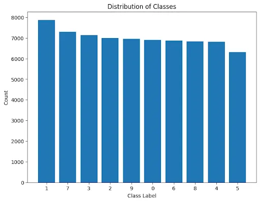
Here we can see that there is enough data for every class of the data, ensuring lesser chances of the class imbalance problem. Also, we can see how the count of different classes is distributed throughout the data. Now let’s move towards the independent variable.

Let’s check for the null values on the independent data side.

#countoing missing value in the data

missing_values_count = X.isnull().apply(pd.value_counts)

counts = missing_values_count.sum(axis=1)

counts.plot(kind=’bar’)

Output:

 

Here we can see that there is no null value in the data. Low lets try to draw one of the image from the data.

import matplotlib.pyplot as plt

# Plot the first number in X

plt.imshow(X.iloc[0].values.reshape(28, 28), cmap=’gray’)

plt.axis(‘off’)

plt.show()

Output:

Here we can see how the images inside the data is bounded. Now our term is to preprocess the data because the model package defined under the sklearn library requires preprocessing data to model it.

Data Preprocessing

As we know that the values under this data are numerical, we would need to standardise and normalise the data. We do this to save the model from becoming overfitted.

X = X/255.0

from sklearn.preprocessing import scale

X_scaled = scale(X)

The above code helps us normalise and scale the data. Now we can split the data.

from sklearn.model_selection import train_test_split

X_train, X_test, y_train, y_test = train_test_split(X_scaled, y, test_size = 0.3, train_size = 0.2 ,random_state = 10)

After splitting the data, we are ready to model the data.

Data Modelling

To model this data using the SVM algorithm, we are going to use the model package given by the sklearn library under the SVM package.

from sklearn.svm import SVC

first_model = SVC(kernel = ‘rbf’)

first_model.fit(X_train, y_train)

Output:

This is how we can simply call and fit the model on the data. Let’s validate its results.

Model Evaluation

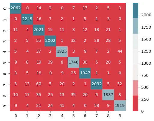
Till now, we have seen the data analysis, preprocessing and modelling. Now once we have the trained model, we need to validate the process we followed is optimum or not. To do so we can use a confusion matrix and accuracy. Using the below code, we can visualise our model performance as a confusion matrix.

y_pred = first_model.predict(X_test)

import seaborn as sns

# accuracy

from sklearn.metrics import confusion_matrix, accuracy_score

print(“accuracy:”, accuracy_score(y_true=y_test, y_pred=y_pred), “n”)

# Generate the confusion matrix

cm = confusion_matrix(y_test, y_pred)

cmap = sns.diverging_palette(10, 220, sep=80, n=7)

# Plot the confusion matrix as a heatmap

sns.heatmap(cm,annot=True, cmap=cmap ,fmt=’g’)

Output:

Here we can see that the model we have defined is more than 94% accurate, and also, in the confusion matrix there are no major classes predicted wrong by the models. Now we can also check for the classification report of the model.

from sklearn.metrics import classification_report

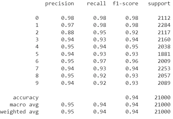
print(classification_report(y_test, y_pred

Output:

 

Here we can see that model is performing great, and its accuracy is 94%. Now let’s conclude this topic as we have got an optimum model for MNIST image classification.

Conclusion

In this article, we have seen how an SVM model can perform with real-life data when there is a huge number of features. As explained in the last article, the SVM is high performing when the feature of the data is higher than the data points, and there are rare fields where such data generates. So if we have a huge number of data features in a dataset and the task is classification, SVM becomes an optimum option to model the data that also requires less calculation and power than the other statistical machine learning algorithms.

About DSW

DSW, specializing in Artificial Intelligence and Data Science, provides platforms and solutions for leveraging data through AI and advanced analytics. With offices located in Mumbai, India, and Dublin, Ireland, the company serves a broad range of customers across the globe.

Our mission is to democratize AI and Data Science, empowering customers with informed decision-making. Through fostering the AI ecosystem with data-driven, open-source technology solutions, we aim to benefit businesses, customers, and stakeholders and make AI available for everyone.

Our flagship platform ‘UnifyAI’ aims to streamline the data engineering process, provide a unified pipeline, and integrate AI capabilities to support businesses in transitioning from experimentation to full-scale production, ultimately enhancing operational efficiency and driving growth.

In real-life data science and machine learning scenarios, we often deal with large-size datasets. Dealing with tremendously large datasets is challenging and at least significantly difficult to cause a bottleneck in modelling an algorithm.

When we go deeper, we find the number of features in a dataset makes data large in size. However, not always a large number of instances comes with a large number of features, but this is not the point of discussion here. It is also very often that in a high-dimensional dataset, we find many irrelevant or insignificant features because they contribute less or zero when applying data for predictive modelling. It has also been seen that they can impact modelling negatively. Here are some possible impacts these features have in efficient predictive modelling:

• Unnecessary memory and resource allocation are required for such features and make the process slow.
• Machine learning algorithm performs poorly because such features act as noise for them.
• Modelling data with high-dimensional features takes more time than data with low dimensions.

So, feature selection comes here as a saviour here, which is also an economical solution. In this article we are going to talk about the following topics:

Table of content

• What is Feature Selection?
• Feature Selection Methods
• Difference Between Filter, Wrapper and Embedded Methods for Feature Selection
• A Case Study in Python

What is Feature Selection?

Feature selection is the process of extracting or selecting a subset of features from a dataset having a large number of features. While extracting features from a dataset, we should consider their potential level before applying them for machine learning and statistical modelling.

The motive behind this procedure is to reduce the number of input features used for final modelling. At the same time selected feature should be the most important one to model. Talking about the impact, this procedure simplifies the machine learning model and improves accuracy and efficiency. Many times it also saves models from overfitting.

The point which is noticeable here is that feature selection is different from features engineering in some cases, because feature engineering refers to the process of creating new features or variables that are not explicitly present in the original dataset but may be useful in improving the performance of a model. On the other hand, feature selection is concerned with selecting the most relevant features from a given set of features.

However, there are different methods of feature selection, such as filter wrapper methods and embedded methods. Let’s take a look at the basic methods of feature selection.

Feature Selection Methods

In general feature selection method can be classified into three main methods:

Filter methods: these methods help us in selecting important features by evaluating the statistical properties of dependent and independent features, such as correlation, mutual information, or significance tests, independent of the learning algorithm. The below image explains further methods.

Some examples of this type of method are as follows

• Correlation-based Feature Selection (CFS): In this type of feature selection procedure, we consider the correlation evaluation between the dependent and independent features of data. Here we select the subsets of features based on the highest correlation with the target feature.
• Mutual Information: this method is similar to the CFS method, but it works based on the mutual information evaluation between the dependent and independent variables. Based on the mutual information evaluation, we eliminated features from data that have the lowest mutual information with the target variables.

Principal Component Analysis (PCA): Using this method, we reduce the dimension of the data and try to get a smaller set of principal components that explain most of the variance in the data.

Wrapper methods: In this method, we evaluate the performance of the model with different subsets of features. Here we use a specific algorithm to select the best subset of features. This type of method assesses the performance of a predictive model using a particular subset of features and iteratively searches for the best subset of features that results in the highest performance. The below picture gives us a glimpse of wrapper methods of feature selection:

Some examples of wrapper methods for feature selection are as follows:

• Forward Selection: in this method, any selected algorithm starts modelling data with an empty set of features and iteratively adds one feature at a time, evaluating the performance of the predictive model at each step. This process continues until the algorithm uses a desired number of features or until it not gains an optimal performance.
• Backward Elimination: We can think of this method as the opposite of the forward selection method, where it starts with a whole set of features and removes one feature in every iteration. This process continues until the algorithm uses a desired number of features or until it not gains an optimal performance.
• Recursive Feature Elimination (RFE): With this method, we recursively remove the features from the model based on their importance in the modelling procedure, and it ends where we get optimal results from the model or optimal subset of features.

Embedded Methods: As the name suggests, this type of feature selection method perform feature selection and model training simultaneously. In embedded methods, feature selection is performed during model training, with the aim of selecting the most relevant features for the specific model being used. There are a variety of algorithms such as decision trees, support vector machines, and linear regression, that can work with embedded feature selection methods.

Some examples of embedded methods for feature selection include LASSO (Least Absolute Shrinkage and Selection Operator) and Ridge Regression, where these methods perform regularisation by shrinking the coefficients of the less important features to zero and selecting the subset of features that have non-zero coefficients for linear regression, and Decision Trees with pruning for decision tree models.

Difference Between Filter, Wrapper and Embedded Methods for Feature Selection

In the above, we have seen the basic classification of different feature selection methods, and in difference, we can say that these methods belong to three broad categories. Some basic differences between these methods are as follows:

• Filter methods are independent of any specific machine learning model, whereas Wrapper methods are used to improve the performance of any specific machine learning model. Embedded methods select features during the model training process.
• Filter methods rank the features based on their ability to explain the target variable, Wrapper methods evaluate the relevance of features based on their ability to improve the performance of a specific ML model, whereas Embedded methods incorporate the feature selection process into the model training process itself with the aim of selecting the most relevant features for the specific model being used.
• Filter methods may not always identify the optimal subset of features when there is insufficient data to capture the statistical correlations between the features. In contrast, Wrapper and Embedded methods can provide the best subset of features as they evaluate the performance of a model with different subsets of features in iterations or during the time of training exhaustively.
• Wrapper methods are generally more computationally expensive and time taking than filter methods, while embedded methods can be more efficient than wrapper methods.
• Using features selected by wrapper methods in the final machine learning model may increase the risk of overfitting as the model has already been trained using those features in multiple iterations. When talking about embedded methods, the risk of overfitting with embedded feature selection methods depends on the complexity of the model being trained, the quality of the selected features, and the regularisation techniques used. In contrast, filter methods typically select a subset of features based on their relevance to the target variable without directly incorporating the model performance into the selection process.

Good enough!

Now take a look at the basic implementation of feature selection.

A Case Study in Python

Here, we are going to use Pima Indians Diabetes Dataset, whose objective is to diagnostically predict whether or not a patient has diabetes based on certain diagnostic measurements included in the dataset.

Let’s start by importing some basic libraries, modules and packages that we will need on the way to feature selection.

import pandas as pd

import numpy as np

from sklearn.feature_selection import SelectKBest, chi2, RFE

from sklearn.linear_model import LogisticRegression

Now, let’s import the dataset.

data = pd.read_csv(“/content/diabetes.csv”)

After successfully importing the data, let’s take a look at some of the rows.

data.head()

In the above, we can see that eight features in the dataset are told about the patient being diabetic in the form of 0 and 1. Talking about the missing values on the data, we can see the NAN values are replaced by 0. Anyone can deduce this by knowing the definition of the columns because it is impractical to have zero values in body mass and insulin columns.

Now we can convert these data into numpy array form to get faster computation.

array = data.values

#features

X = array[:,0:8]

#target

Y = array[:,8]

Filter Method

Here, we will perform a chi-squared statistical test for features with non-negative values and will select three features from the data. The chi-squared test belongs to the filter method of feature selection.

test = SelectKBest(score_func=chi2, k=4)

fit = test.fit(X, Y)

print(fit.scores_)

Output:

Here, we can see the Chi-square score of the features. Now we can transform important features. Let’s take a look.

features = fit.transform(X)

print(features[0:5,:])

Output:

Here are the four selected features of the dataset based on the chi-square test.

Wrapper Method

Next, we will take a look at the implementation of Recursive Feature Elimination, which belongs to the wrapper method of feature selection. In the above, we have explained how this method works.

We know that the wrapper methods are used to improve the performance of any specific machine learning model so here we will work with the logistic regression model.

model = LogisticRegression()

rfe = RFE(model, n_features_to_select=3, step=3)

fit = rfe.fit(X, Y)

Output:

Here, we have applied the RFE feature selection for the logistic regression model. Lets see the results now.

print(“Num Features: n”, fit.n_features_)

print(“Selected Features: n”, fit.support_)

print(“Feature Ranking: n”, fit.ranking_)

Output:

Here we can see the ranking of the features of the dataset, also in the second output we can see which features are supporting the most. Now let’s take a look at the embedded method.

Embedded Method

Here, we will use the lasso regression for feature selection. Basically, it is a regression technique which adds a penalty term to the cost function of regression that encourages sparsity in the coefficients.

In practice, Lasso can be used as a feature selection method by fitting a Lasso regression model on a dataset and examining the resulting coefficient vector to determine which features are important. Features with non-zero coefficients are considered important, while those with zero coefficients can be discarded.

Let’s make an object of lasso regression and fit the data on it.

# Fit Lasso model

lasso = Lasso(alpha=0.1)

lasso.fit(X, Y)

Let’s check the importance of all the features

# Extract coefficients and print feature importance

coef = np.abs(lasso.coef_)

print(“Feature importance:n”)

for i in range(len(data.columns:

print(f”{data.columns[i]}: {coef[i]}”)

Output:

Here we can see the ranking of important features when we use the lasso regression.

Final words

Till now, we have discussed feature selection, different methods of feature selection and a basic implementation of feature selection using the Python programming language. Because of this article, we get to know that the subject feature selection is itself a big course, so in future articles, we will take a look at more details of this topic where, one by one, we will explain all the variants of the feature selection method.

About DSW

DSW, specializing in Artificial Intelligence and Data Science, provides platforms and solutions for leveraging data through AI and advanced analytics. With offices located in Mumbai, India, and Dublin, Ireland, the company serves a broad range of customers across the globe.

Our mission is to democratize AI and Data Science, empowering customers with informed decision-making. Through fostering the AI ecosystem with data-driven, open-source technology solutions, we aim to benefit businesses, customers, and stakeholders and make AI available for everyone.

Our flagship platform ‘UnifyAI’ aims to streamline the data engineering process, provide a unified pipeline, and integrate AI capabilities to support businesses in transitioning from experimentation to full-scale production, ultimately enhancing operational efficiency and driving growth.

In the field of data science, the deployment and operation of AI/ML models can be a challenging task due to various reasons, like increasing the amount of data. To overcome these challenges, the concept of ModelOps was introduced in the early 2020s. ModelOps encompasses a set of practices and processes that not only aid in the creation of models but also in the deployment of them in a scalable and flexible manner. This focus on ModelOps has become increasingly important as organizations strive to effectively utilize machine learning models in their operations. ModelOps has become a rapidly growing field as a result. So let’s take an introductory dive into the subject and understand what ModelOps is and how it is becoming the point of attraction for AI and ML developers.

What is ModelOps?

ModelOps can be referred to as the management and operationalisation of ML models within the ML processing of any organisation. As many big organisations are using a load of Ai use cases, it becomes a compulsion to develop these use cases so that they can have higher speed and scalability and improved quality and accuracy. Like DevOps, MLOps and DataOps, ModelOps is also a set of practices that involves the enhancement of a wide range of activities, such as machine learning model development, testing, deployment, monitoring, and maintenance.

According to Gartner,” ModelOps (or AI model operationalisation) is focused primarily on the governance and life cycle management of a wide range of operationalised artificial intelligence (AI) and decision models, including machine learning, knowledge graphs, rules, optimisation, linguistic and agent-based models. Core capabilities include continuous integration/continuous delivery (CI/CD) integration, model development environments, champion-challenger testing, model versioning, model store and rollback.”

The aim behind applying ModelOps in the development process is to ensure that ML models are better developed and used efficiently in real-world applications. This helps organisations to enhance their capability to generate business value from their ML models and investments. ModelOps is a relatively newer term in the technology space, but it is becoming way more important because organisations are relying more on machine learning models for critical business processes.

Talking about the challenge that ModelOps helps organisations overcome, mainly in the deployment of machine learning models, such as difficulties in the reproduction of final results, less transparency, slow iteration times etc., the ultimate goal of applying ModelOps is to maximise the value of organisations investment on machine learning.

Component of ModelOps

The components of ModelOps can be segregated into the following groups:

Model development: this section may include the tools for extracting prepared and feature-engineered data from data sources and for model selection and training.

Model deployment: this section contains tools for model packaging, model and architecture provisioning, and model deployment to the production environment.

Model Monitoring: this section includes tools for monitoring and capturing model performance and data and model drift while interfacing for model retraining.

Model maintenance: this section includes tools for managing models, storing model versions, model documentation and requirement and model retraining place.

Model governance: this section includes a set of rules to control access, implement policies and track activity for models and their results.

Collaboration and communication: these are a set of rules and management skills to make better collaboration between data scientists and DevOps teams, communication between stakeholders, and integration with other tools and systems.

Benefits of ModelOps

However, the term ModelOps is inspired by the concept of DevOps and MLOps, but its adoption ensures:

• Developers are provided with CI/CD(continuous integration / continuous delivery)
• Improved Development Environment
• Better Testing
• Controlled model versioning

One can think of ModelOps as a part of MLops, which mainly focuses on keeping deployed models ready to involve in continuous model developing or retraining and synchronized deployment. There are several benefits of ModelOps, such as:

• Improved model quality: ModelOps helps ensure that machine learning models are reliable, accurate, and consistent by introducing processes for testing, validation, and monitoring the performance of the models.
• Faster model deployment: ModelOps automates the deployment process, reducing the time it takes to get models into production and increasing the speed at which new models can be deployed.
• Better model governance: ModelOps provides a framework for managing the lifecycle of machine learning models, including versioning, auditing, and regulatory compliance.
• Increased agility: ModelOps enables organizations to respond quickly to changes in business requirements or market conditions by allowing teams to update or replace models in a timely manner.
• Improved operational efficiency: ModelOps streamlines the operations of machine learning models, reducing manual effort and increasing the scalability and reliability of the models.

Difference between ModelOps and MLOps

Often organisation uses the terms ModelOps and MlOps interchangeably, but when going into the deeper section, we find subtle differences between the two.

In one of our articles, we explored the MLOps profoundly and learned that it is a broader term that helps in processing the entire lifecycle of AI/ML models, from processing data to deployment and management of the models. This term consists of an entire set of practices for data processing, data management building, testing, deploying and monitoring AI/ML models.

On the other hand, ModelOps only focuses on the operational aspects of AI/ML models. ModelOps includes practices for processes such as model management, deployment, monitoring, and maintenance. Involving these practices in development ensures that the models are deployed, monitored, and maintained efficiently in production.

In conclusion, we can say that ModelOps practices are more focused on operational aspects of AI/ML models, while MLOps is a broader term that includes ModelOps as a subset that majorly focuses on the deployment, maintaining and monitoring the AI/ML models.

Is MLOps a combination of DataOps and ModelOps?

In the above section, we learned that ModelOps is a subset of MLOps that focuses only on operational aspects of AI/ML models, but due to this article, we have learned that DataOps is a set of practices and technologies that are designed to address the challenges of managing and processing large volumes of data in a fast-paced and constantly changing environment.

So we can say that the terms MLOps, ModelOps and DataOps are related but distinct concepts that are all part of the broader term of data science and machine learning.

The focus point of DataOps is to ensure that data is high-quality, accessible, and secure and that the process of moving data through the pipeline is efficient and reliable.

On the other hand, ModelOps is a set of practices, tools and technologies focusing on streamlining the model development and deployment process, making it more efficient and reliable while also ensuring that models are continuously monitored and updated to reflect changing data and business needs.

Here we can say that MLOps is a combination of DataOps and ModelOps that is focused specifically on the machine learning workflow, from data collection to model deployment. While DataOps and ModelOps are both important components of MlOps, they are not the same. Rather MLOps is an umbrella term that encompasses both DataOps and ModelOps, as well as other practices and technologies that are specific to the machine learning workflow.

Implementing a comprehensive data-driven strategy that involves the use of DataOps, ModelOps, and MLOps can be a complex and challenging task for organizations. This is because it often requires the collaboration of different teams with different areas of expertise and can involve the integration of a variety of technologies and processes.

UnifyAI, DSW’s platform, is an ideal solution to overcome the challenges and intricacies that organizations face when implementing DataOps, ModelOps, and MLOps simultaneously. Collaboration and communication among different teams are necessary to address the complexities. UnifyAI integrates MLOps, DataOps, and ModelOps to create a culture of collaboration and knowledge-sharing among teams. This allows organizations to achieve a comprehensive data-driven strategy and reduces the dependence on a large number of teams and members by offering all necessary technologies and tools aligned with best practices for implementing smooth ML workflows.

About DSW

DSW, specializing in Artificial Intelligence and Data Science, provides platforms and solutions for leveraging data through AI and advanced analytics. With offices located in Mumbai, India, and Dublin, Ireland, the company serves a broad range of customers across the globe.

Our mission is to democratize AI and Data Science, empowering customers with informed decision-making. Through fostering the AI ecosystem with data-driven, open-source technology solutions, we aim to benefit businesses, customers, and stakeholders and make AI available for everyone.

Our flagship platform ‘UnifyAI’ aims to streamline the data engineering process, provide a unified pipeline, and integrate AI capabilities to support businesses in transitioning from experimentation to full-scale production, ultimately enhancing operational efficiency and driving growth.